WorldView Stereopair Selection: SpaceNet UCSD Example

This notebook documents the stereo-pair selection analysis used to choose three candidate pairs from the IARPA CORE3D / SpaceNet UCSD dataset for the companion processing notebook worldview_spacenet_ucsd_stereo.ipynb.

The goal is to rigorously scan all 35 WV3 scenes available for UCSD, compute pair geometry with asp_plot.stereopair_metadata_parser, and select three pairs with stable imaging geometry for the mixed campus-and-coastal-hills terrain at UCSD.

Background: stable imaging geometry

Jeong, J. & Kim, T. (2016), Comparison of positioning accuracy of a rigorous sensor model and two rational function models for weak stereo geometry, ISPRS Journal of Photogrammetry and Remote Sensing 82(8): 625–633 — https://www.sciencedirect.com/science/article/abs/pii/S0099111216301021:

Stable imaging geometry, in addition to a precise sensor model, is also necessary to achieve detailed mapping. The stability of the imaging geometry can be expressed by the values of three angles: the convergence, bisector elevation (BIE), and asymmetry angles. The convergence angle reflects the base-to-height ratio; the BIE angle describes the obliqueness of the epipolar plane; the asymmetry angle specifies the level of symmetry between the left and right observation rays. In the ideal imaging geometry, the epipolar plane would be orthogonal (90° BIE angle) and symmetric (0° asymmetry angle) to the ground plane, to avoid accuracy degradation.

So the ideal is BIE → 90° and asymmetry → 0°. In this notebook these two angles are treated as secondary tiebreakers: they only move a pair up or down the ranking when they are notably far from ideal (BIE ≲ 70°, asymm ≳ 12°).

Convergence target for this scene

Purely urban stereo analyses cite ~5–15° as the ideal convergence range — see Aguilar, M.Á. et al. (2019), 3D modelling of urban structures from very high resolution satellite imagery: a comparative analysis of convergence angle effect, European Journal of Remote Sensing, 52(sup1): 1–13 — https://www.tandfonline.com/doi/full/10.1080/22797254.2018.1551069#abstract. Small convergence reduces occlusion and matching failures on tall, steep-sided building facades.

But UCSD is a mixed landscape — campus and residential blocks plus deep coastal valleys, cliffs, and hills toward Mount Soledad / Torrey Pines. Pure low-convergence pairs under-constrain height recovery over the natural, lower-slope portions. Rules of thumb used in this notebook:

• Urban-only scenes: ~5–15° is ideal (minimizes building occlusion).

• Natural / low-slope terrain: higher convergence (≳ 25°) is beneficial — the larger base-to-height ratio improves vertical precision where occlusion is not the limiting factor.

• Mixed urban + natural scenes (UCSD): ~15–25° is a practical middle ground.

Scoring priority

Priority	Criterion	Direction
Primary	Convergence angle	Target 15–25°
Primary	ROI overlap (% + containment of the processing ROI)	Larger, full containment required
Primary	Temporal separation |Δt| (days)	Smaller
Primary	Solar geometry similarity (|Δsun_el|, |Δsun_az|, UTC hour delta)	Smaller
Primary	Off-nadir angle per scene	Smaller (finer GSD, less oblique)
Primary	Sensor consistency	Prefer WV3 + WV3
Secondary	BIE angle	Tiebreaker; penalize only if ≲ 70°
Secondary	Asymmetry angle	Tiebreaker; penalize only if ≳ 12°

---

Setup

This notebook only downloads the small *.tar metadata archives (~2 MB each) — not the ~800 MB *.NTF images — because all we need to assess pair geometry is the XML camera metadata. Files go to /tmp/ucsd_scene_selection/ and are cleaned up at the end.

import os
import shutil
import subprocess
import tempfile
from itertools import combinations
from pathlib import Path

import contextily as ctx
import geopandas as gpd
import matplotlib.pyplot as plt
import numpy as np
import pandas as pd
from shapely.geometry import box

from asp_plot.stereopair_metadata_parser import StereopairMetadataParser
from asp_plot.utils import get_xml_tag

WORK_DIR = Path("/tmp/ucsd_scene_selection")
TAR_DIR = WORK_DIR / "tars"
XML_DIR = WORK_DIR / "xmls"
FLAT_DIR = WORK_DIR / "flat_xmls"
for d in (WORK_DIR, TAR_DIR, XML_DIR, FLAT_DIR):
    d.mkdir(parents=True, exist_ok=True)

S3_PREFIX = "s3://spacenet-dataset/Hosted-Datasets/CORE3D-Public-Data/Satellite-Images/UCSD/WV3/PAN/"

# Region of interest for processing — a 3 x 3 km window over the UCSD campus,
# Mount Soledad, and Torrey Pines. UTM Zone 11N (EPSG:32611): xmin ymin xmax ymax.
# All candidate pairs must fully cover this ROI.
T_PROJWIN = (476000, 3635600, 479000, 3638600)
UTM_EPSG = 32611

---

1. Discover all WV3 scenes on S3

The SpaceNet CORE3D UCSD bucket contains 35 WV3 panchromatic scenes in WV3/PAN/. We list them with aws s3 ls --no-sign-request and capture the .tar filenames.

result = subprocess.run(
    ["aws", "s3", "ls", "--no-sign-request", S3_PREFIX],
    capture_output=True, text=True, check=True,
)
tar_names = sorted(
    line.split()[-1]
    for line in result.stdout.strip().splitlines()
    if line.endswith(".tar")
)
print(f"Found {len(tar_names)} tar archives on S3.")
print("First 3:")
for t in tar_names[:3]:
    print(" ", t)

Found 35 tar archives on S3.
First 3:
  01JAN16WV031300016JAN01185802-P1BS-500647760070_01_P001_________AAE_0AAAAABPABN0.tar
  05JAN15WV031300015JAN05183041-P1BS-500647758090_01_P001_________AAE_0AAAAABPABS0.tar
  06FEB15WV031300015FEB06184344-P1BS-500647761030_01_P001_________AAE_0AAAAABPABQ0.tar

2. Download metadata archives and extract XMLs

Each .tar archive is ~2 MB. The .NTF imagery (~800 MB each) is not downloaded — pair assessment uses only the XML camera models.

for name in tar_names:
    dst = TAR_DIR / name
    if dst.exists() and dst.stat().st_size > 0:
        continue
    subprocess.run(
        ["aws", "s3", "--no-sign-request", "cp",
         f"{S3_PREFIX}{name}", str(dst), "--only-show-errors"],
        check=True,
    )
print(f"Tars on disk: {len(list(TAR_DIR.glob('*.tar')))}")

# Extract each tar (idempotent — tar -x overwrites unchanged files)
for tar in TAR_DIR.glob("*.tar"):
    subprocess.run(["tar", "xf", str(tar), "-C", str(XML_DIR)], check=True)

# The archives nest deeply; pull the *P1BS*.XML files out into a flat dir
for xml in XML_DIR.rglob("*P1BS*.XML"):
    if "PAN" in str(xml):
        shutil.copy(xml, FLAT_DIR / xml.name)
print(f"P1BS XMLs flattened: {len(list(FLAT_DIR.glob('*.XML')))}")

Tars on disk: 35

P1BS XMLs flattened: 35

3. Extract per-scene metadata

We use StereopairMetadataParser.get_id_dict(catid, xml) to parse each XML into a dict with sensor, date, viewing geometry, solar geometry, GSD, footprint polygon, and ephemeris. The parser is instantiated with a throwaway 2-XML directory (just to satisfy __init__); we call get_id_dict manually for each of the 35 scenes — this is N-scene-safe and avoids the built-in dg_mosaic path the class takes when it sees > 2 XMLs in a single directory (intended for mosaicking tiles of one scene).

# Set up a dummy parser — get_id_dict() and pair_dict() only need `self` for
# helper methods (xml2poly, getEphem_gdf, etc.) and do not use self.image_list.
_dummy = tempfile.mkdtemp()
xmls_sorted = sorted(FLAT_DIR.glob("*.XML"))
for x in xmls_sorted[:2]:
    shutil.copy(x, _dummy)
parser = StereopairMetadataParser(_dummy)

scene_dicts = []
rows = []
for x in xmls_sorted:
    catid = get_xml_tag(str(x), "CATID")
    d = parser.get_id_dict(catid, str(x), geteph=True)
    scene_dicts.append(d)
    rows.append({
        "catid": d["catid"],
        "sensor": d["sensor"],
        "date": d["date"],
        "off_nadir": d["meanoffnadirviewangle"],
        "sat_az": d["meansataz"],
        "sat_el": d["meansatel"],
        "sun_az": d["meansunaz"],
        "sun_el": d["meansunel"],
        "gsd_m": d["meanproductgsd"],
        "cloud": d["cloudcover"],
    })

scene_df = pd.DataFrame(rows).sort_values("date").reset_index(drop=True)
print(f"{len(scene_df)} scenes parsed.")
scene_df

35 scenes parsed.

	catid	sensor	date	off_nadir	sat_az	sat_el	sun_az	sun_el	gsd_m	cloud
0	104001000365CA00	WV03	2014-10-27 18:25:10.483175	17.0	161.3	71.2	157.8	41.6	0.33	0.00
1	10400100039E7C00	WV03	2014-10-28 18:40:08.733775	23.2	263.8	64.4	162.6	42.3	0.36	0.00
2	104001000496A100	WV03	2014-11-09 18:29:48.722375	1.1	184.8	88.6	160.8	38.1	0.31	0.01
3	1040010004B41D00	WV03	2014-11-22 18:34:28.860375	13.0	227.6	75.6	162.6	35.1	0.32	0.00
4	10400100047BBB00	WV03	2014-11-28 18:29:01.304775	14.7	172.6	73.7	161.0	33.5	0.33	0.00
5	10400100057DD500	WV03	2014-12-23 18:22:36.081975	24.1	132.4	63.3	157.2	30.3	0.36	0.00
6	1040010005843100	WV03	2015-01-05 18:30:41.419775	8.2	146.0	80.8	157.4	31.2	0.31	0.00
7	10400100071D8800	WV03	2015-01-24 18:35:47.652175	16.3	199.2	71.8	155.5	34.3	0.33	0.00
8	1040010007713300	WV03	2015-02-06 18:43:44.791775	22.6	239.3	65.0	155.5	38.2	0.36	0.00
9	1040010007A3D100	WV03	2015-02-11 18:23:49.684775	24.3	81.0	63.2	149.0	37.7	0.36	0.00
10	1040010007A93700	WV03	2015-02-12 18:39:26.584775	8.4	268.3	80.8	153.3	39.6	0.32	0.00
11	1040010007CA4D00	WV03	2015-02-24 18:31:34.272575	12.9	140.4	75.7	148.9	42.7	0.32	0.00
12	1040010009673900	WV03	2015-03-21 18:29:22.415375	18.7	74.4	69.5	143.4	51.7	0.34	0.00
13	104001000A269C00	WV03	2015-04-10 18:46:41.829375	23.4	233.6	64.0	145.7	61.3	0.36	0.00
14	104001000A3D7E00	WV03	2015-04-28 18:31:36.260975	17.2	114.0	71.0	133.0	64.9	0.33	0.00
15	104001000B230500	WV03	2015-04-29 18:47:09.198975	22.3	232.4	65.3	140.0	67.4	0.35	0.00
16	104001000FCC8E00	WV03	2015-07-26 18:37:42.672575	24.4	40.3	63.2	122.7	68.1	0.36	0.01
17	104001000FBADE00	WV03	2015-07-27 18:54:00.322775	23.7	246.4	63.7	130.8	70.7	0.36	0.00
18	104001000F0EB300	WV03	2015-08-08 18:46:09.037575	21.7	197.5	65.8	133.0	67.3	0.35	0.00
19	104001000F2DF400	WV03	2015-08-14 18:41:10.903575	11.7	51.3	77.3	133.9	65.3	0.32	0.00
20	1040010010339E00	WV03	2015-08-27 18:48:56.191775	19.9	211.1	67.9	144.6	63.2	0.34	0.00
21	104001001159EA00	WV03	2015-09-28 18:57:51.547575	23.6	262.8	64.0	162.2	53.8	0.36	0.00
22	10400100130B9B00	WV03	2015-10-23 18:53:12.033775	21.7	221.9	66.0	166.1	44.8	0.35	0.00
23	1040010013426E00	WV03	2015-11-17 18:48:02.317375	21.9	187.1	65.6	166.4	37.1	0.35	0.00
24	10400100140ED300	WV03	2015-11-23 18:43:04.334775	19.2	152.1	68.7	164.9	35.5	0.34	0.00
25	10400100149C7200	WV03	2015-11-29 18:37:32.745575	24.2	77.2	63.3	163.2	33.9	0.36	0.00
26	1040010014AF5E00	WV03	2015-12-13 18:58:48.063975	22.6	247.3	65.0	167.8	33.2	0.36	0.00
27	10400100162B0400	WV03	2015-12-18 18:38:06.476375	23.5	84.2	64.0	161.8	31.7	0.36	0.00
28	1040010016570500	WV03	2015-12-25 18:49:02.014575	20.4	185.0	67.3	163.7	32.1	0.34	0.00
29	1040010016C57700	WV03	2015-12-31 18:43:43.612175	18.4	144.9	69.6	161.5	31.9	0.34	0.00
30	1040010016091700	WV03	2016-01-01 18:58:02.512575	24.2	328.7	63.5	165.1	32.8	0.36	0.00
31	10400100179C8D00	WV03	2016-01-26 18:53:38.536575	21.9	204.9	65.7	160.0	36.1	0.35	0.00
32	1040010017A92D00	WV03	2016-02-08 18:58:10.215175	21.7	230.3	65.9	159.4	39.9	0.35	0.00
33	1040010018921400	WV03	2016-02-14 18:52:56.516575	21.8	197.9	65.8	157.0	41.3	0.35	0.00
34	10400100190C5100	WV03	2016-02-20 18:47:27.440975	12.1	143.1	76.5	154.4	42.8	0.32	0.00

4. Enumerate all unique pairs and compute geometry metrics

With 35 scenes we have $\binom{35}{2} = 595$ candidate pairs. For each pair we compute (via parser.pair_dict):

• conv_ang — convergence angle (degrees)

• bh_ratio — base-to-height ratio (derived from convergence)

• bie_ang — bisector elevation angle (degrees; ideal 90°)

• asymm_ang — asymmetry angle (degrees; ideal 0°)

• inter_km2 — intersection-footprint area

• inter_perc_min — minimum of (% of each scene that is intersected)

Plus manually-computed acquisition-condition deltas:

• dt_days — temporal separation (calendar days)

• delta_sun_el, delta_sun_az — solar geometry differences (degrees; az uses circular distance)

• tod_hour_delta — time-of-day (UTC hour) delta — sun-shadow-direction proxy

• roi_contained — does the intersection polygon fully contain the 3 × 3 km processing ROI?

roi_utm_poly = box(*T_PROJWIN)
roi_latlon_poly = (
    gpd.GeoDataFrame(geometry=[roi_utm_poly], crs=f"EPSG:{UTM_EPSG}")
    .to_crs("EPSG:4326")
    .geometry.iloc[0]
)

pair_rows = []
for d1, d2 in combinations(scene_dicts, 2):
    if d1["date"] > d2["date"]:
        d1, d2 = d2, d1
    pairname = f"{d1['catid']}_{d2['catid']}"
    p = parser.pair_dict(d1, d2, pairname)

    dt_days = p["dt"].total_seconds() / 86400.0
    delta_sun_el = abs(d1["meansunel"] - d2["meansunel"])
    dsun_az = abs(d1["meansunaz"] - d2["meansunaz"])
    delta_sun_az = min(dsun_az, 360 - dsun_az)
    hour1 = d1["date"].hour + d1["date"].minute / 60.0
    hour2 = d2["date"].hour + d2["date"].minute / 60.0
    dh = abs(hour1 - hour2)
    tod_hour_delta = min(dh, 24 - dh)

    if p["intersection"] is not None:
        roi_contained = p["intersection"].contains(roi_latlon_poly)
        inter_area = p["intersection_area"]
        inter_perc = min(p["intersection_area_perc"])
    else:
        roi_contained = False
        inter_area = None
        inter_perc = None

    pair_rows.append({
        "pairname": pairname,
        "catid1": d1["catid"], "catid2": d2["catid"],
        "sensor1": d1["sensor"], "sensor2": d2["sensor"],
        "date1": d1["date"], "date2": d2["date"],
        "dt_days": round(dt_days, 2),
        "conv_ang": p["conv_ang"],
        "bh_ratio": p["bh"],
        "bie_ang": p["bie"],
        "asymm_ang": p.get("asymmetry_angle"),
        "inter_km2": inter_area,
        "inter_perc_min": inter_perc,
        "roi_contained": roi_contained,
        "off_nadir1": d1["meanoffnadirviewangle"],
        "off_nadir2": d2["meanoffnadirviewangle"],
        "delta_sun_el": round(delta_sun_el, 2),
        "delta_sun_az": round(delta_sun_az, 2),
        "tod_hour_delta": round(tod_hour_delta, 2),
    })

pair_df = pd.DataFrame(pair_rows)
print(f"Computed {len(pair_df)} pairs.")
print(f"Pairs fully containing the ROI: {pair_df.roi_contained.sum()}")
print(f"Pairs with convergence in 15–25°: {((pair_df.conv_ang >= 15) & (pair_df.conv_ang <= 25)).sum()}")

Computed 595 pairs.
Pairs fully containing the ROI: 595
Pairs with convergence in 15–25°: 163

5. Filter and score

Filters

1. The intersection polygon must fully contain the 3 × 3 km ROI (roi_contained == True).

2. Convergence must not be missing.

Scoring

Smaller score → better. Weights reflect the priority table from the intro: convergence dominates, followed by solar geometry and temporal separation. BIE and asymmetry are applied as penalty flags that activate only when notably bad (BIE < 70° or asymm > 12°), so they don’t dominate a well-behaved pair’s ranking.

score = 3.0 · conv_penalty            # 0 inside [15, 25°], else distance from that band
      + 0.15 · dt_days
      + 0.30 · |Δsun_el|
      + 0.10 · |Δsun_az|
      + 0.10 · mean(off_nadir1, off_nadir2)
      + 5.0  · (bie_ang < 70)
      + 5.0  · (asymm_ang > 12)

def conv_penalty(c):
    if 15 <= c <= 25:
        return 0.0
    return float(min(abs(c - 15), abs(c - 25)))

scored = pair_df[pair_df.roi_contained & pair_df.conv_ang.notna()].copy()

scored["conv_penalty"] = scored["conv_ang"].apply(conv_penalty)
scored["bie_flag"] = (scored["bie_ang"] < 70).astype(int)
scored["asymm_flag"] = (scored["asymm_ang"] > 12).astype(int)

scored["score"] = (
    3.0  * scored["conv_penalty"]
  + 0.15 * scored["dt_days"]
  + 0.30 * scored["delta_sun_el"]
  + 0.10 * scored["delta_sun_az"]
  + 0.10 * scored[["off_nadir1", "off_nadir2"]].mean(axis=1)
  + 5.0  * scored["bie_flag"]
  + 5.0  * scored["asymm_flag"]
)

scored = scored.sort_values("score").reset_index(drop=True)
print(f"Candidates after filtering: {len(scored)}")

display_cols = [
    "pairname", "dt_days", "conv_ang", "bie_ang", "asymm_ang",
    "inter_perc_min", "delta_sun_el", "delta_sun_az",
    "tod_hour_delta", "off_nadir1", "off_nadir2", "score",
]
scored[display_cols].head(15)

Candidates after filtering: 595

	pairname	dt_days	conv_ang	bie_ang	asymm_ang	inter_perc_min	delta_sun_el	delta_sun_az	tod_hour_delta	off_nadir1	off_nadir2	score
0	1040010018921400_10400100190C5100	6.00	19.60	72.98	10.40	91.80	1.5	2.6	0.08	21.8	12.1	3.3050
1	104001000365CA00_104001000496A100	13.00	17.52	79.95	9.84	90.13	3.5	3.0	0.07	17.0	1.1	4.2050
2	1040010007A93700_1040010007CA4D00	11.99	21.21	84.31	2.73	94.82	3.1	4.4	0.13	8.4	12.9	4.2335
3	104001000496A100_10400100047BBB00	19.00	14.93	81.16	8.64	94.32	4.6	0.2	0.00	1.1	14.7	5.2500
4	1040010007A3D100_1040010007CA4D00	13.01	22.84	71.73	11.63	81.98	5.0	0.1	0.13	24.3	12.9	5.3215
5	1040010004B41D00_10400100047BBB00	6.00	14.14	76.31	2.08	97.25	1.6	1.6	0.08	13.0	14.7	5.5050
6	10400100071D8800_1040010007A93700	19.00	17.14	78.38	7.00	93.51	5.3	2.2	0.07	16.3	8.4	5.8950
7	1040010005843100_10400100071D8800	19.00	14.61	77.55	8.35	93.48	3.1	1.9	0.08	8.2	16.3	6.3650
8	1040010016C57700_10400100179C8D00	26.01	22.19	70.38	4.07	94.79	4.2	1.5	0.17	18.4	21.9	7.3265
9	104001000365CA00_1040010004B41D00	26.01	18.36	75.94	4.01	96.78	6.5	4.8	0.15	17.0	13.0	7.8315
10	10400100179C8D00_10400100190C5100	25.00	21.31	73.42	9.73	90.64	6.7	5.6	0.10	21.9	12.1	8.0200
11	1040010007713300_1040010007A93700	6.00	17.49	73.31	15.40	82.63	1.4	2.2	0.07	22.6	8.4	8.0900
12	104001000496A100_1040010004B41D00	13.00	13.41	82.27	7.53	92.06	3.0	1.8	0.08	1.1	13.0	8.5050
13	1040010007CA4D00_1040010009673900	25.00	19.47	75.19	5.76	90.43	9.0	5.5	0.03	12.9	18.7	8.5800
14	10400100057DD500_1040010005843100	13.01	17.88	72.14	17.48	80.20	0.9	0.2	0.13	24.1	8.2	8.8565

6. Visualize the ranked candidates

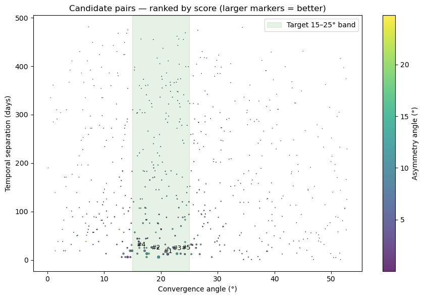
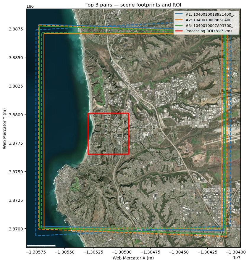
Two views:

1. Scatter — convergence angle vs. temporal separation, colored by asymmetry, sized by inverse score. The 15–25° target band is shaded.

2. Map — scene footprints for the top 3 pairs over an Esri WorldImagery basemap with the ROI highlighted.

fig, ax = plt.subplots(figsize=(9, 6))
sc = ax.scatter(
    scored["conv_ang"], scored["dt_days"],
    c=scored["asymm_ang"], cmap="viridis",
    s=60 * np.clip(1 / (scored["score"] + 0.5), 0, 5),
    alpha=0.8, edgecolor="k", linewidth=0.3,
)
cb = plt.colorbar(sc, ax=ax, label="Asymmetry angle (°)")
ax.axvspan(15, 25, color="green", alpha=0.10, label="Target 15–25° band")
for i in range(min(5, len(scored))):
    row = scored.iloc[i]
    ax.annotate(f"#{i+1}", (row["conv_ang"], row["dt_days"]),
                textcoords="offset points", xytext=(6, 6), fontsize=9)
ax.set_xlabel("Convergence angle (°)")
ax.set_ylabel("Temporal separation (days)")
ax.set_title("Candidate pairs — ranked by score (larger markers = better)")
ax.legend(loc="upper right")
plt.tight_layout()
plt.show()

fig, ax = plt.subplots(figsize=(9, 9))

top3_idx = scored.index[:3]
colors = ["tab:blue", "tab:orange", "tab:green"]

for i, (idx, color) in enumerate(zip(top3_idx, colors)):
    row = scored.loc[idx]
    g1 = next(d["geom"] for d in scene_dicts if d["catid"] == row["catid1"])
    g2 = next(d["geom"] for d in scene_dicts if d["catid"] == row["catid2"])
    for g, style in [(g1, "--"), (g2, "-")]:
        gdf = gpd.GeoDataFrame(geometry=[g], crs="EPSG:4326").to_crs(3857)
        gdf.boundary.plot(ax=ax, color=color, linestyle=style, linewidth=2,
                          label=f"#{i+1}: {row['pairname'][:17]}…" if style == "-" else None)

roi_gdf = gpd.GeoDataFrame(geometry=[roi_utm_poly], crs=f"EPSG:{UTM_EPSG}").to_crs(3857)
roi_gdf.boundary.plot(ax=ax, color="red", linewidth=2.5, label="Processing ROI (3×3 km)")

ctx.add_basemap(ax, crs=3857, source=ctx.providers.Esri.WorldImagery, attribution_size=0)
ax.set_title("Top 3 pairs — scene footprints and ROI")
ax.legend(loc="upper right", fontsize=9)
ax.set_xlabel("Web Mercator X (m)")
ax.set_ylabel("Web Mercator Y (m)")
plt.tight_layout()
plt.show()

7. Selected pairs

The three pairs carried forward into the processing notebooks were chosen from the ranked candidates to span the 15–25° convergence band while keeping temporal separation, solar geometry, and BIE/asymmetry all in good shape. They are all same-sensor (WV3 + WV3) and all fully contain the 3 × 3 km processing ROI.

Pair folder / notebook suffix	catid1 × catid2	Conv (°)	|Δt| (d)	BIE (°)	Asymm (°)	Overlap %	|Δsun_el| (°)
14deg_6d	1040010004B41D00 × 10400100047BBB00	14.14	6	76.3	2.1	97.3	1.6
18deg_13d	104001000365CA00 × 104001000496A100	17.52	13	80.0	9.8	90.1	3.5
21deg_12d	1040010007A93700 × 1040010007CA4D00	21.21	12	84.3	2.7	94.8	3.1

The 18° pair has a noticeably asymmetric geometry (asymm 9.8°, just under the 12° flag threshold) — it’s retained because its convergence sits at the middle of the urban-ideal band and gives us a useful mid-convergence comparison, but we’ll note when reviewing its DEM whether the asymmetry shows up in the residuals.

Processing notebooks (same cropped ROI, same reference DEM, same pipeline):

• worldview_spacenet_ucsd_stereo_14deg_6d.ipynb

• worldview_spacenet_ucsd_stereo_18deg_13d.ipynb

• worldview_spacenet_ucsd_stereo_21deg_12d.ipynb

selected_pairs = [
    ("14deg_6d",  "1040010004B41D00", "10400100047BBB00"),
    ("18deg_13d", "104001000365CA00", "104001000496A100"),
    ("21deg_12d", "1040010007A93700", "1040010007CA4D00"),
]
for tag, c1, c2 in selected_pairs:
    row = scored[
        scored.apply(lambda r: frozenset({r.catid1, r.catid2}) == frozenset({c1, c2}), axis=1)
    ].iloc[0]
    print(f"{tag:10s}  rank={scored.index.get_loc(row.name)+1:3d}  "
          f"conv={row.conv_ang:5.2f}°  bie={row.bie_ang:5.2f}°  asymm={row.asymm_ang:5.2f}°  "
          f"dt={row.dt_days:5.1f}d  overlap={row.inter_perc_min:5.1f}%  "
          f"Δsun_el={row.delta_sun_el:4.1f}°")

14deg_6d    rank=  6  conv=14.14°  bie=76.31°  asymm= 2.08°  dt=  6.0d  overlap= 97.2%  Δsun_el= 1.6°
18deg_13d   rank=  2  conv=17.52°  bie=79.95°  asymm= 9.84°  dt= 13.0d  overlap= 90.1%  Δsun_el= 3.5°
21deg_12d   rank=  3  conv=21.21°  bie=84.31°  asymm= 2.73°  dt= 12.0d  overlap= 94.8%  Δsun_el= 3.1°

8. Processing outcomes: DEM-vs-ICESat-2 comparison

We ran the full ASP stereo workflow on the three scene-selected candidate pairs from section 7.

For each resulting DEM we compared against ICESat-2 ATL06-SR ground-track points over the ROI. The table below summarizes pre- and post-pc_align height-residual statistics, compiled from a one-off offline run.

Stat columns:

• n_icesat: ATL06-SR points retained after 3σ outlier filtering

• median_dh_pre_m / nmad_dh_pre_m: median and NMAD of ATL06-SR minus DEM before pc_align (meters)

• translation_mag_m (|T|): magnitude of the 3D rigid translation applied by pc_align

• median_dh_post_m / nmad_dh_post_m: same percentiles after alignment

pc_align only solves for a rigid translation, so it is the post-alignment NMAD that gives the cleanest read on intrinsic DEM quality: the median collapses toward zero by construction, and pre-alignment bias reflects absolute positioning rather than DEM geometry.

pair	catid1	catid2	dt (d)	conv (°)	asymm (°)	B/H	n ICESat-2	median pre (m)	NMAD pre (m)	|T| (m)	median post (m)	NMAD post (m)	selected
14deg_6d	1040010004B41D00	10400100047BBB00	6	14.1	2.1	0.25	1053	2.05	2.01	1.99	0.09	1.97
18deg_13d	104001000496A100	104001000365CA00	13	17.5	9.8	0.31	1024	−1.23	1.77	1.42	−0.05	1.77
21deg_12d	1040010007A93700	1040010007CA4D00	12	21.2	2.7	0.37	977	−7.53	1.63	8.00	0.05	1.53	yes

Why 21deg_12d was selected

• Lowest post-alignment NMAD (1.53 m) of the three pairs — the DEM is the most internally consistent after a rigid shift is removed.

• Convergence angle of 21.2° sits comfortably in the middle of the 15–25° band targeted in section 5.

• Asymmetry of 2.7° means both scenes contribute comparable geometric weight to the stereo solution.

• The 8.0 m translation magnitude is the largest of the three, but the NMAD improvement confirms this reflects a fixed absolute bias rather than internal DEM distortion; pc_align removes it cleanly.

The canonical processing notebook worldview_spacenet_ucsd_stereo.ipynb uses this pair (1040010007A93700 × 1040010007CA4D00) and its companion PDF report is at WorldView_UCSD-asp-plot-report.pdf.

9. Clean up

Remove all temporary tar/XML files. Only the XML metadata lives under /tmp/, so nothing outside the working directory is affected. Re-running this notebook will re-download the ~70 MB of tars from S3.

shutil.rmtree(WORK_DIR, ignore_errors=True)
print(f"Removed {WORK_DIR}: {not WORK_DIR.exists()}")

Removed /tmp/ucsd_scene_selection: True