WorldView Stereopair Processing: SpaceNet Atlanta Example (No Mapprojection)

This notebook is a variant of the SpaceNet Atlanta WorldView stereo notebook that skips the mapprojection step and runs parallel_stereo directly on the bundle-adjusted (raw) WV2 images using --alignment-method affineepipolar. The final section compares the ICESat-2 histograms of the resulting DEM against the mapprojected version, illustrating the impact of mapprojection on the output.

The same stereopair is used as in the mapprojected notebook:

catid	tile	off-nadir (°)
1030010002B7D800	P002	14.0	left
1030010003CAF100	P002	10.6	right

Pair geometry (from StereopairMetadataParser):

• Convergence angle: 21.77°

• Base-to-height ratio: 0.38

• BIE angle: 81.57° (ideal 90°)

• Asymmetry angle: 2.34° (ideal 0°)

• Temporal separation: 0 days (same-pass MVS collect, 2009-12-22)

• Intersection overlap: 82.4%

Why a no-mapprojection example?

For WorldView imagery, mapprojecting the inputs onto a reference DEM before stereo is the recommended workflow — it minimizes disparity search ranges and produces cleaner DEMs. This notebook demonstrates the alternative path (--alignment-method affineepipolar on the raw bundle-adjusted images) so users can see the difference in DEM quality and to provide a more representative example for situations where a reference DEM is unavailable or unreliable.

This notebook reuses the bundle adjustment from the mapprojected notebook (ba/) and writes its stereo outputs to a separate stereo_no_mapproj/ subdirectory, so both runs can coexist in the same processing directory for direct comparison.

---

Processing Overview

• Data Retrieval — Download WorldView-2 tiles from AWS S3 (same as mapprojected notebook)

• CCD Artifact Correction — Apply wv_correct to fix WV2 sensor artifacts (same)

• Reference DEM Preparation — Copernicus 30m DEM with WGS84 ellipsoid heights (same; used for difference plots only)

• Bundle Adjustment — Reuse outputs from the mapprojected notebook (ba/)

• Stereo Processing (no mapprojection) — Run parallel_stereo with --alignment-method affineepipolar on the raw bundle-adjusted images, writing to stereo_no_mapproj/

• Visualization with asp_plot — Plots, ICESat-2 comparison, PDF report

• Histogram Comparison — Side-by-side ICESat-2 histograms with vs. without mapprojection

---

Data Retrieval

The full catalogue of WV2 CATIDs and the pair-selection analysis is documented in the companion notebook worldview_spacenet_atlanta_stereo_scene_selection.ipynb. This notebook processes the 22deg_0d pair chosen there.

Download Commands

The SpaceNet Atlanta raw L1B images are in s3://spacenet-dataset/AOIs/AOI_6_Atlanta/metadata/<CATID>/<workorder>_<PXXX>_PAN/. Download only the specific tiles needed for this pair:

$ mkdir -p atlanta_stereo_22deg_0d/images
$ cd atlanta_stereo_22deg_0d/images

# Download left image tile: 1030010002B7D800 P002
$ aws s3 --no-sign-request sync \
  s3://spacenet-dataset/AOIs/AOI_6_Atlanta/metadata/1030010002B7D800/ \
  aws/1030010002B7D800/ \
  --exclude "*" --include "*P002_PAN/*"

# Download right image tile: 1030010003CAF100 P002
$ aws s3 --no-sign-request sync \
  s3://spacenet-dataset/AOIs/AOI_6_Atlanta/metadata/1030010003CAF100/ \
  aws/1030010003CAF100/ \
  --exclude "*" --include "*P002_PAN/*"

Copy the TIF and XML files to the working directory with short names:

$ cd atlanta_stereo_22deg_0d
$ cp images/aws/1030010002B7D800/*P002_PAN/*P1BS*P002.TIF 1030010002B7D800_P002.tif
$ cp images/aws/1030010002B7D800/*P002_PAN/*P1BS*P002.XML 1030010002B7D800_P002.xml
$ cp images/aws/1030010003CAF100/*P002_PAN/*P1BS*P002.TIF 1030010003CAF100_P002.tif
$ cp images/aws/1030010003CAF100/*P002_PAN/*P1BS*P002.XML 1030010003CAF100_P002.xml

Note on Tiling

Each Atlanta CATID is delivered as multiple tiles (P001, P002, P003). For this pair we use individual tiles (P002 from 1030010002B7D800 and P002 from 1030010003CAF100) that each fully contain the airport ROI. Mosaicking with dg_mosaic is not needed.

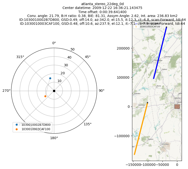
Stereo Geometry Analysis

Before processing, it’s useful to analyze the stereo acquisition geometry to verify the convergence angle and other geometric properties. We use asp_plot to visualize the geometry from the XML camera metadata:

# Set the base directory for your processing
directory = "~/Desktop/asp-plot-examples/atlanta_stereo_22deg_0d/"

from asp_plot.stereo_geometry import StereoGeometryPlotter

sgp = StereoGeometryPlotter(directory)
utm_code = sgp.get_pair_utm_epsg()
map_crs = f"EPSG:{utm_code}"
scene_bounds = sgp.get_scene_bounds()

print(f"Auto-detected UTM projection: {map_crs}")
print(f"Scene extent (lon/lat): {scene_bounds[0]:.6f} {scene_bounds[1]:.6f} {scene_bounds[2]:.6f} {scene_bounds[3]:.6f}")

sgp.dg_geom_plot()

Auto-detected UTM projection: EPSG:32616
Scene extent (lon/lat): -84.492554 33.591823 -84.307826 33.724071

Satellite Position and Orientation Data

The XML camera metadata also contains ephemeris (position/velocity) and attitude (orientation quaternion) data reported by the satellite during acquisition. Visualizing this data can help assess the quality of the raw metadata before ASP processing.

sgp.satellite_position_orientation_plot()

In the above plot:

• Top row (Position Covariance): A map showing the satellite’s path over the ground during image capture, colored by how uncertain the satellite’s reported position is (in meters). Lower values mean the satellite knows where it is more precisely.

• Middle row (Roll / Pitch / Yaw): Shows how the satellite’s pointing deviates from its expected nadir-pointing orientation over time. Roll is rotation around the flight direction, pitch is rotation around the cross-track axis, and yaw is rotation around the nadir axis. Values near zero mean the satellite is pointing straight down. These are computed by comparing the raw attitude quaternions against a reference orientation estimated from the satellite’s orbital position and velocity.

• Bottom row (Attitude Covariance Trace): Shows how uncertain the satellite’s orientation knowledge is over time. Lower values mean the satellite is more confident about which direction it’s pointing. Spikes or jumps indicate moments of less reliable pointing knowledge, which could affect image quality in those portions of the scene.

---

CCD Artifact Correction

WorldView-2 imagery has subpixel CCD boundary misalignments. The SpaceNet Atlanta data was processed in 2019 (before the May 2022 improvement), so wv_correct is required:

$ cd atlanta_stereo_22deg_0d

$ wv_correct 1030010002B7D800_P002.tif 1030010002B7D800_P002.xml 1030010002B7D800_P002_corr.tif
$ wv_correct 1030010003CAF100_P002.tif 1030010003CAF100_P002.xml 1030010003CAF100_P002_corr.tif

The *_corr.tif corrected images are used for all subsequent processing steps.

---

Processing Configuration

$ cd atlanta_stereo_22deg_0d

# Target spatial reference system (UTM Zone 16N for Atlanta)
$ t_srs="EPSG:32616"

# Output resolution — use the more nadir image's meanProductGSD
$ tr=0.481

# Reference DEM filename (WGS84 ellipsoid heights, projected to UTM)
$ reference_dem_fn="ref/cop30_atlanta_wgs84_utm.tif"

Image-space crop window for the airport ROI

Without mapprojection, ASP cannot use the UTM t_projwin from the mapprojected notebook directly — that is a ground-coordinate crop. The equivalent in image space is --left-image-crop-win <ulx> <uly> <width> <height>, which restricts parallel_stereo to a pixel window of the left image (ASP automatically computes the matching window on the right).

We derived an image-space crop window for the same airport ROI by inverse-projecting the four corners of t_projwin="735685 3722295 741350 3727695" (UTM Zone 16N) back through the left tile’s RPC camera model, taking the bounding box of the resulting pixel coordinates, and adding a 500-pixel buffer for safety. This can be done in a few lines using GDAL’s RPC transformer:

from osgeo import gdal, osr

gdal.UseExceptions()

utm = osr.SpatialReference(); utm.ImportFromEPSG(32616)
geo = osr.SpatialReference(); geo.ImportFromEPSG(4326)
for srs in (utm, geo):
    srs.SetAxisMappingStrategy(osr.OAMS_TRADITIONAL_GIS_ORDER)
ct = osr.CoordinateTransformation(utm, geo)

ds = gdal.Open("1030010002B7D800_P002.tif")  # has RPC metadata
tx = gdal.Transformer(ds, None, ["METHOD=RPC", "RPC_HEIGHT=300"])

xs, ys = [], []
for x, y in [(735685, 3722295), (741350, 3722295),
             (741350, 3727695), (735685, 3727695)]:
    lon, lat, _ = ct.TransformPoint(x, y)
    _, (px, py, _) = tx.TransformPoint(1, lon, lat, 300.0)
    xs.append(px); ys.append(py)

ulx, uly = int(min(xs)) - 500, int(min(ys)) - 500
lrx, lry = int(max(xs)) + 500, int(max(ys)) + 500
print(f"--left-image-crop-win {ulx} {uly} {lrx - ulx} {lry - uly}")
# => --left-image-crop-win 5879 13107 12981 11894

This restricts stereo to roughly 154 Mpx (vs ~1 Gpx for the full overlap), bringing the runtime closer to the mapprojected notebook’s airport-only run.

---

Reference DEM Preparation

A reference DEM is required for mapprojecting the input images and validating the output DEM. We use the Copernicus 30m GLO-30 DEM.

Download Copernicus DEM with Ellipsoid Heights

$ cd atlanta_stereo_22deg_0d

$ python /path/to/your/fetch_dem/download_global_DEM.py \
  -demtype COP30_E \
  -extent "$scene_bounds" \
  -out_fn "$reference_dem_fn" \
  -out_proj "$t_srs" \
  -apikey [YOUR_OPEN_TOPOGRAPHY_API_KEY]

---

Bundle Adjustment

This notebook reuses the bundle adjustment outputs from the mapprojected notebook. If you have not already run that notebook, run the bundle adjustment step there first (the ba/ outputs are independent of mapprojection):

$ cd atlanta_stereo_22deg_0d

$ bundle_adjust \
  --threads 8 \
  --ip-per-image 10000 \
  --tri-weight 0.1 \
  --tri-robust-threshold 0.1 \
  --camera-weight 0 \
  1030010002B7D800_P002_corr.tif 1030010003CAF100_P002_corr.tif \
  1030010002B7D800_P002.xml 1030010003CAF100_P002.xml \
  -o ba/run

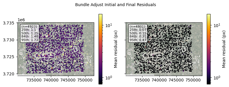
Bundle Adjustment Results

Visualize the bundle adjustment results to verify the optimization reduced reprojection errors:

from asp_plot.bundle_adjust import ReadBundleAdjustFiles, PlotBundleAdjustFiles
import contextily as ctx

# Define subdirectories
bundle_adjust_directory = "ba/"
stereo_directory = "stereo_no_mapproj/"

# Map configuration (map_crs was auto-detected in the geometry cell above)
ctx_kwargs = {
    "crs": map_crs,
    "source": ctx.providers.Esri.WorldImagery,
    "attribution_size": 0,
    "alpha": 0.5,
}

# Read bundle adjustment residuals
ba_files = ReadBundleAdjustFiles(directory, bundle_adjust_directory)
resid_initial_gdf, resid_final_gdf = ba_files.get_initial_final_residuals_gdfs(residuals_in_meters=True)

# Plot residuals before and after optimization
plotter = PlotBundleAdjustFiles(
    [resid_initial_gdf, resid_final_gdf],
    lognorm=True,
    title="Bundle Adjust Initial and Final Residuals"
)
plotter.plot_n_gdfs(
    column_name="mean_residual",
    cbar_label="Mean residual (px)",
    map_crs=map_crs,
    **ctx_kwargs
)

---

Stereo Processing (No Mapprojection)

We run parallel_stereo directly on the bundle-adjusted, CCD-corrected (but not mapprojected) images, using --alignment-method affineepipolar so ASP performs an internal affine epipolar alignment for the stereo correlation. We pass the airport-ROI crop window derived above so the run is comparable in area (and runtime) to the mapprojected notebook:

$ cd atlanta_stereo_22deg_0d

$ parallel_stereo \
  --stereo-algorithm asp_mgm --subpixel-mode 9 \
  --processes 2 --threads 4 --alignment-method affineepipolar \
  --left-image-crop-win 5879 13107 12981 11894 \
  --bundle-adjust-prefix ba/run \
  1030010002B7D800_P002_corr.tif 1030010003CAF100_P002_corr.tif \
  1030010002B7D800_P002.xml 1030010003CAF100_P002.xml \
  stereo_no_mapproj/run

# Generate ~1.9 m DEM (~4x the native input GSD)
$ point2dem --tr 1.9 --t_srs "$t_srs" --errorimage stereo_no_mapproj/run-PC.tif

# Difference map vs. reference DEM
$ geodiff stereo_no_mapproj/run-DEM.tif "$reference_dem_fn" -o stereo_no_mapproj/run_vs_ref

Compared with the mapprojected stereo command in the companion notebook, the differences are:

• The input image filenames are the bundle-adjusted CCD-corrected tiles (*_corr.tif) instead of the mapprojected tiles (*_corr_map.tif).

• --alignment-method affineepipolar replaces --alignment-method none.

• --left-image-crop-win (image pixels) replaces --t_projwin (UTM coordinates) — the derivation above maps one to the other.

• The reference DEM is not passed as the final positional argument (that argument is only used by mapprojected stereo).

• Output is written to stereo_no_mapproj/ so it does not overwrite the mapprojected stereo run.

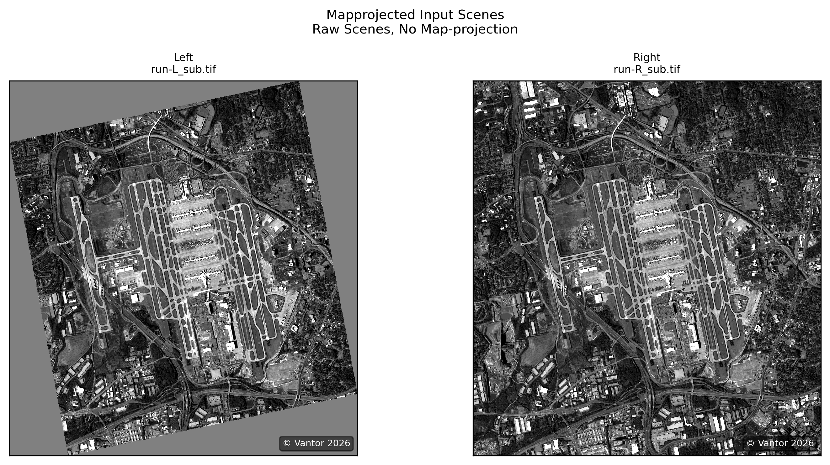
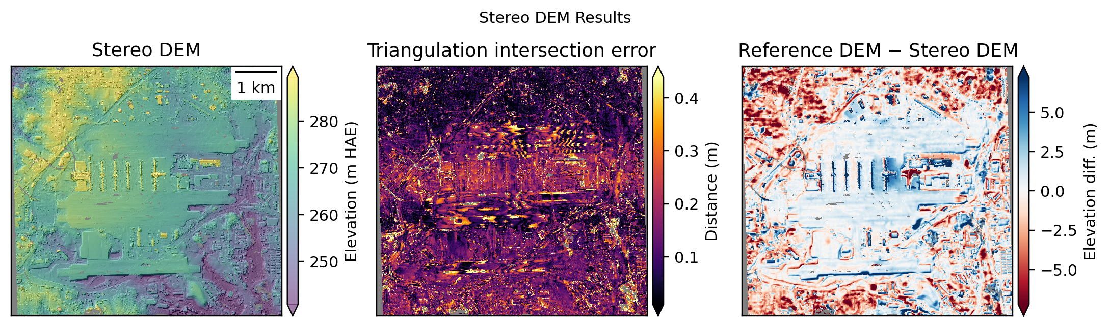
Stereo Results Visualization

Examine the stereo processing outputs to assess DEM quality:

from asp_plot.stereo import StereoPlotter
from asp_plot.scenes import ScenePlotter

# Plot input scenes (mapprojected images)
scene_plotter = ScenePlotter(directory, stereo_directory, title="Mapprojected Input Scenes")
scene_plotter.plot_scenes()

# Plot DEM results
stereo_plotter = StereoPlotter(directory, stereo_directory)
stereo_plotter.title = "Stereo DEM Results"
stereo_plotter.plot_dem_results()

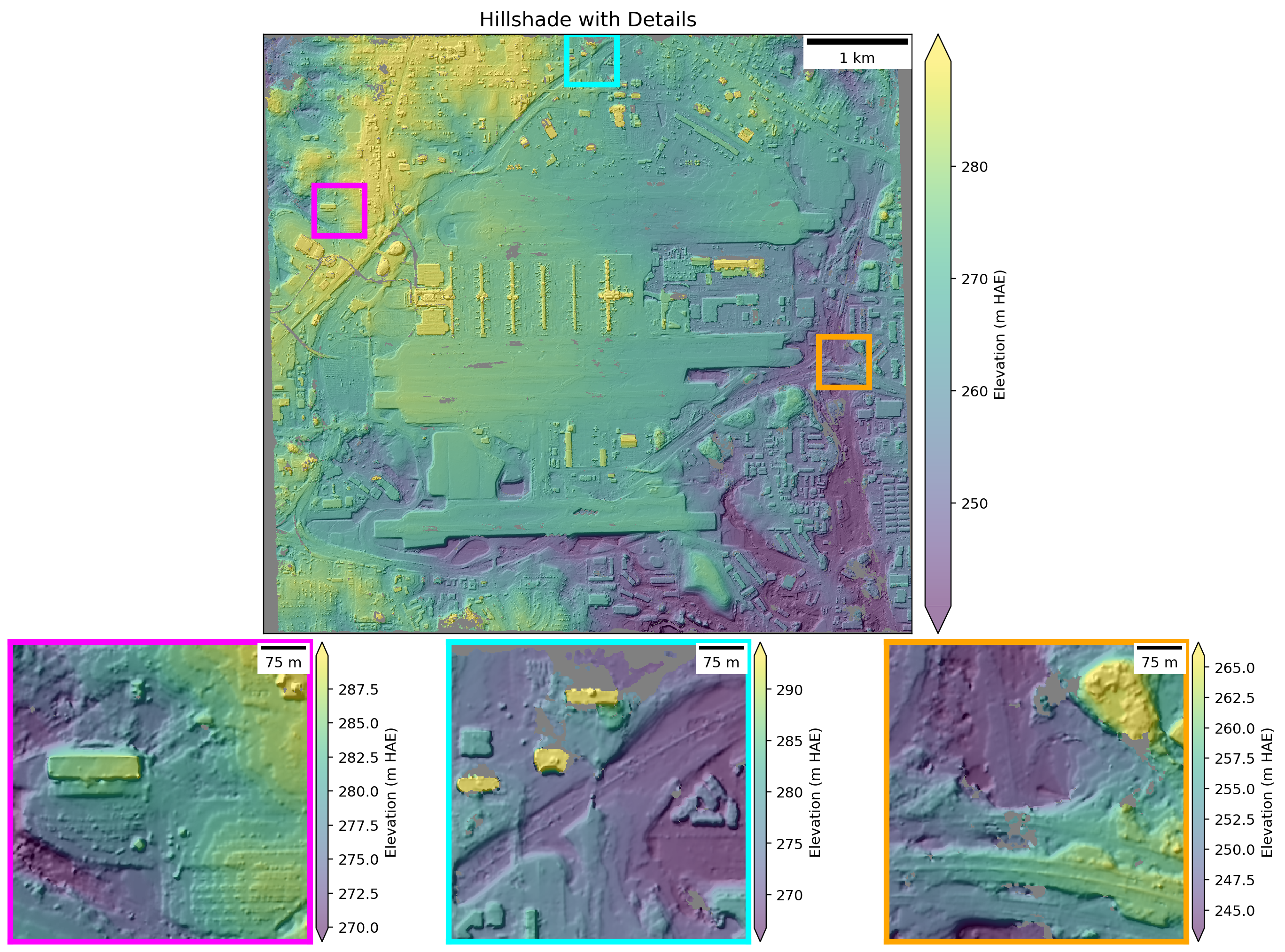
# Plot detailed hillshade with zoom subsets
stereo_plotter.title = "Hillshade with Details"
stereo_plotter.plot_detailed_hillshade(subset_km=0.5)

WARNING:asp_plot.stereo:

No reference DEM found in log files. Please supply the reference DEM you used during stereo processing (or another reference DEM) if you would like to see some difference maps.

ASP DEM: /Users/ben/Desktop/asp-plot-examples/atlanta_stereo_22deg_0d/stereo_no_mapproj/run-DEM.tif

Plotting DEM results. This can take a minute for large inputs.

WARNING:asp_plot.stereo:

Found a DEM of difference: /Users/ben/Desktop/asp-plot-examples/atlanta_stereo_22deg_0d/stereo_no_mapproj/run_vs_ref-diff.tif.
Using that for difference map plotting.

---

Comprehensive Report and ICESat-2 Altimetry Validation

In addition to the inline visualizations above, we can validate the ASP DEM against ICESat-2 ATL06-SR altimetry data. This provides an independent accuracy assessment using satellite laser altimetry.

The sections below demonstrate ICESat-2 comparison and generate a comprehensive PDF report.

Setup

After you have asp_plot installed and ready to use, you can set up the directory and file names:

# Set the base directory for your processing
directory = "~/Desktop/asp-plot-examples/atlanta_stereo_22deg_0d/"

bundle_adjust_directory = "ba/"
stereo_directory = "stereo_no_mapproj/"

Full Report Generation

Generate a comprehensive PDF report:

See the resulting report.

!asp_plot \
  --directory $directory \
  --bundle_adjust_directory $bundle_adjust_directory \
  --stereo_directory $stereo_directory \
  --subset_km 0.5 \
  --report_filename ../../reports/WorldView_Atlanta_without_mapprojection-asp-plot-report.pdf

Processing ASP files in /Users/ben/Desktop/asp-plot-examples/atlanta_stereo_22deg_0d/

WARNING:asp_plot.stereo:

No reference DEM found in log files. Please supply the reference DEM you used during stereo processing (or another reference DEM) if you would like to see some difference maps.



ASP DEM: /Users/ben/Desktop/asp-plot-examples/atlanta_stereo_22deg_0d/stereo_no_mapproj/run-DEM.tif


Using map projection from DEM: EPSG:32616

WARNING:asp_plot.utils:Could not find ('*.[Xx][Mm][Ll]',) in /Users/ben/Desktop/asp-plot-examples/atlanta_stereo_22deg_0d/ba/. Some plots may be missing.
Figure saved to /Users/ben/Desktop/asp-plot-examples/atlanta_stereo_22deg_0d/tmp_asp_report_plots/00.png
Figure saved to /Users/ben/Desktop/asp-plot-examples/atlanta_stereo_22deg_0d/tmp_asp_report_plots/01.png
Figure saved to /Users/ben/Desktop/asp-plot-examples/atlanta_stereo_22deg_0d/tmp_asp_report_plots/02.png
Figure saved to /Users/ben/Desktop/asp-plot-examples/atlanta_stereo_22deg_0d/tmp_asp_report_plots/03.png
Figure saved to /Users/ben/Desktop/asp-plot-examples/atlanta_stereo_22deg_0d/tmp_asp_report_plots/04.png
WARNING:asp_plot.utils:Could not find ('*-mapproj_match_offsets.txt',) in /Users/ben/Desktop/asp-plot-examples/atlanta_stereo_22deg_0d/ba/. Some plots may be missing.


Skipping map-projected residuals plot: 

MapProj Residuals TXT file not found.




WARNING:asp_plot.bundle_adjust:

No reference DEM found in bundle_adjust log. This would only exist if you ran bundle_adjust with the advanced `--mapproj-dem ref_dem.tif` flag. Cannot generate geodiff for /Users/ben/Desktop/asp-plot-examples/atlanta_stereo_22deg_0d/ba/run-initial_residuals_pointmap.csv.




Skipping geodiff plots (requires --mapproj-dem flag in bundle_adjust): 

Geodiff file /Users/ben/Desktop/asp-plot-examples/atlanta_stereo_22deg_0d/ba/run-initial_residuals_pointmap-diff.csv could not be generated. Check that geodiff is installed and a reference DEM was used in bundle_adjust.




Figure saved to /Users/ben/Desktop/asp-plot-examples/atlanta_stereo_22deg_0d/tmp_asp_report_plots/05.png
Plotting DEM results. This can take a minute for large inputs.
WARNING:asp_plot.stereo:

Found a DEM of difference: /Users/ben/Desktop/asp-plot-examples/atlanta_stereo_22deg_0d/stereo_no_mapproj/run_vs_ref-diff.tif.
Using that for difference map plotting.


Figure saved to /Users/ben/Desktop/asp-plot-examples/atlanta_stereo_22deg_0d/tmp_asp_report_plots/06.png
Figure saved to /Users/ben/Desktop/asp-plot-examples/atlanta_stereo_22deg_0d/tmp_asp_report_plots/07.png

Detected planetary body: earth

WARNING:sliderule.sliderule:Warning, this environment is using an outdated client (v5.3.1). The code will run but some functionality supported by the server (v5.4.0) may not be available.
Time filter: 2018-10-14T00:00:00Z to 2026-04-28T00:00:00Z (all available)

ICESat-2 ATL06 request processing for: all
{'poly': [{'lon': -84.4633641359238, 'lat': 33.60976895571787}, {'lon': -84.4633641359238, 'lat': 33.664707653569835}, {'lon': -84.39259416121254, 'lat': 33.664707653569835}, {'lon': -84.39259416121254, 'lat': 33.60976895571787}, {'lon': -84.4633641359238, 'lat': 33.60976895571787}], 't0': '2018-10-14T00:00:00Z', 't1': '2026-04-28T00:00:00Z', 'res': 20, 'len': 40, 'ats': 20, 'fit': {'maxi': 6}, 'cnf': 'atl03_high', 'srt': -1, 'cnt': 10}
Existing file found, reading in: /Users/ben/Desktop/asp-plot-examples/atlanta_stereo_22deg_0d/atl06sr_all.parquet
Filtering ATL06-SR all
  Outlier filter (3σ): all 7921 → 7745 (removed 176)
Figure saved to /Users/ben/Desktop/asp-plot-examples/atlanta_stereo_22deg_0d/tmp_asp_report_plots/08.png
Figure saved to /Users/ben/Desktop/asp-plot-examples/atlanta_stereo_22deg_0d/tmp_asp_report_plots/09.png
Figure saved to /Users/ben/Desktop/asp-plot-examples/atlanta_stereo_22deg_0d/tmp_asp_report_plots/10.png
Figure saved to /Users/ben/Desktop/asp-plot-examples/atlanta_stereo_22deg_0d/tmp_asp_report_plots/11.png

Writing out: /Users/ben/Desktop/asp-plot-examples/atlanta_stereo_22deg_0d/stereo_no_mapproj/run-DEM_pc_align_translated.tif


Wrote out all aligned DEM to /Users/ben/Desktop/asp-plot-examples/atlanta_stereo_22deg_0d/stereo_no_mapproj/run-DEM_pc_align_translated.tif

Figure saved to /Users/ben/Desktop/asp-plot-examples/atlanta_stereo_22deg_0d/tmp_asp_report_plots/12.png
Figure saved to /Users/ben/Desktop/asp-plot-examples/atlanta_stereo_22deg_0d/tmp_asp_report_plots/13.png
Figure saved to /Users/ben/Desktop/asp-plot-examples/atlanta_stereo_22deg_0d/tmp_asp_report_plots/14.png


Report saved to ../../reports/WorldView_Atlanta_without_mapprojection-asp-plot-report.pdf

ICESat-2 Altimetry Validation

Compare the ASP DEM with ICESat-2 ATL06-SR altimetry data:

from asp_plot.altimetry import Altimetry

icesat = Altimetry(
  directory=directory,
  dem_fn=stereo_plotter.dem_fn
)

# Request ATL06-SR data (single "all" processing level)
icesat.request_atl06sr_multi_processing(
    processing_levels=["all"],
    save_to_parquet=True,
)

WARNING:sliderule.sliderule:Warning, this environment is using an outdated client (v5.3.1). The code will run but some functionality supported by the server (v5.4.0) may not be available.

Time filter: 2018-10-14T00:00:00Z to 2026-04-28T00:00:00Z (all available)

ICESat-2 ATL06 request processing for: all
{'poly': [{'lon': -84.4633641359238, 'lat': 33.60976895571787}, {'lon': -84.4633641359238, 'lat': 33.664707653569835}, {'lon': -84.39259416121254, 'lat': 33.664707653569835}, {'lon': -84.39259416121254, 'lat': 33.60976895571787}, {'lon': -84.4633641359238, 'lat': 33.60976895571787}], 't0': '2018-10-14T00:00:00Z', 't1': '2026-04-28T00:00:00Z', 'res': 20, 'len': 40, 'ats': 20, 'fit': {'maxi': 6}, 'cnf': 'atl03_high', 'srt': -1, 'cnt': 10}
Existing file found, reading in: /Users/ben/Desktop/asp-plot-examples/atlanta_stereo_22deg_0d/atl06sr_all.parquet
Filtering ATL06-SR all

# Filter out water bodies
icesat.filter_esa_worldcover(filter_out="water")

No temporal filtering needed for the simplified report workflow. Advanced temporal filtering is still available via:

icesat.predefined_temporal_filter_atl06sr(date=...)
icesat.generic_temporal_filter_atl06sr(select_years=..., select_months=..., ...)

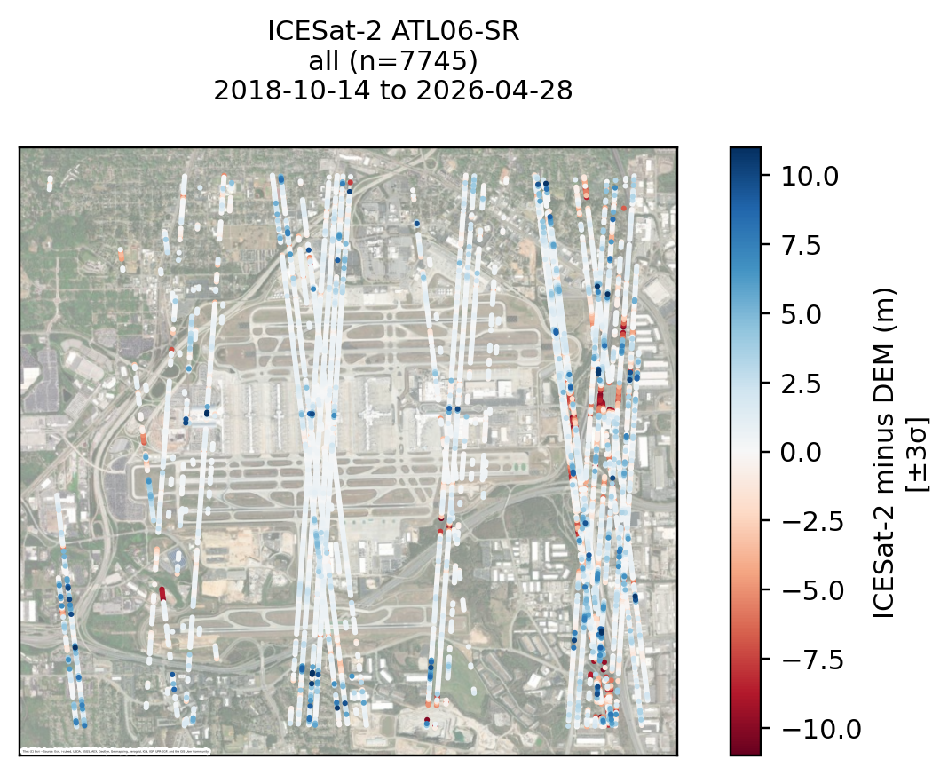
# Map view of ICESat-2 vs DEM differences
icesat.mapview_plot_atl06sr_to_dem(
    key="all",
    map_crs=map_crs,
    **ctx_kwargs,
)

icesat_minus_dem not found in ATL06 dataframe: all. Running differencing first.

  Outlier filter (3σ): all 7921 → 7745 (removed 176)

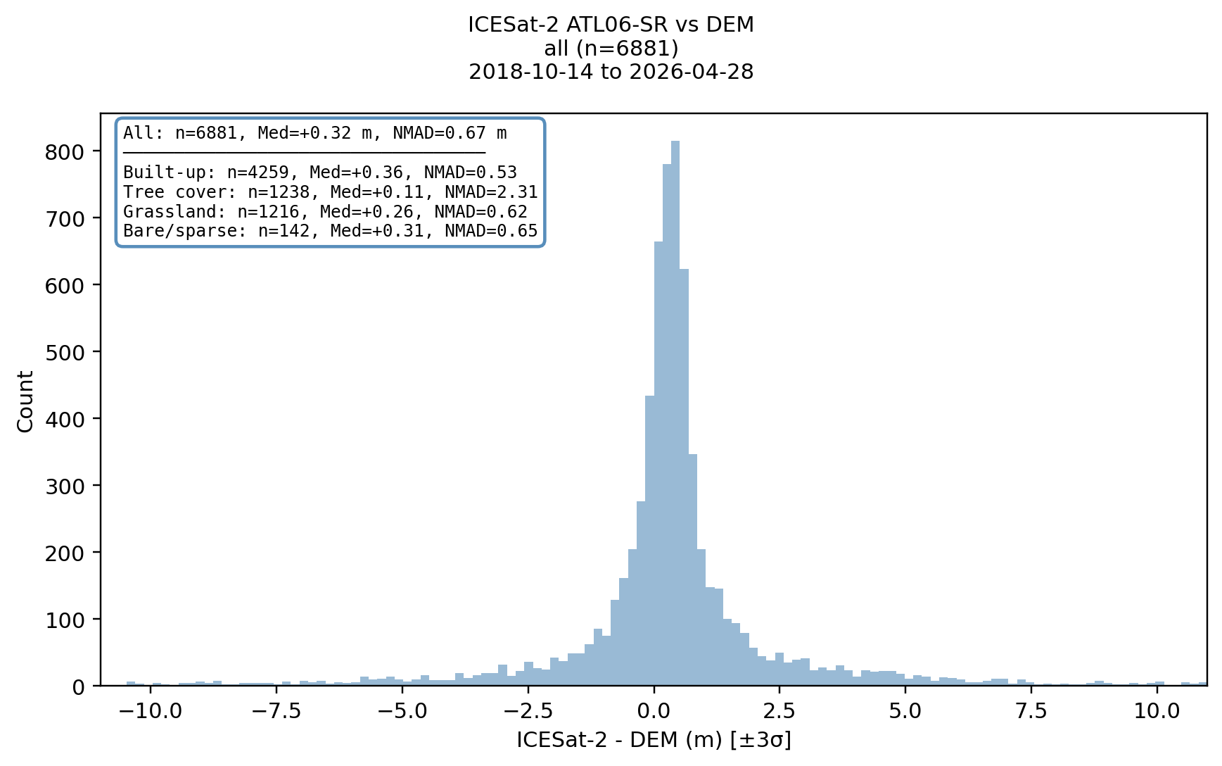
# Histogram with per-landcover-class statistics
icesat.histogram_by_landcover(key="all")

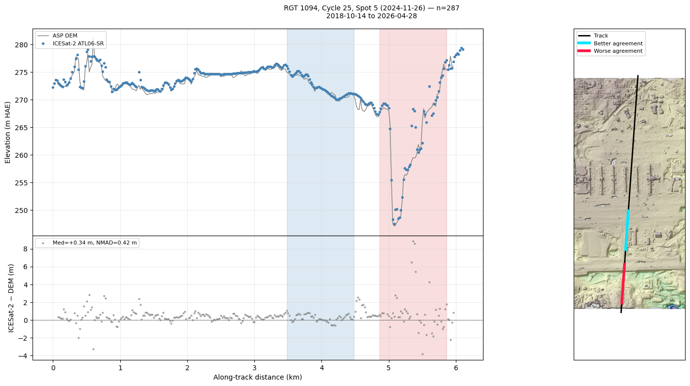
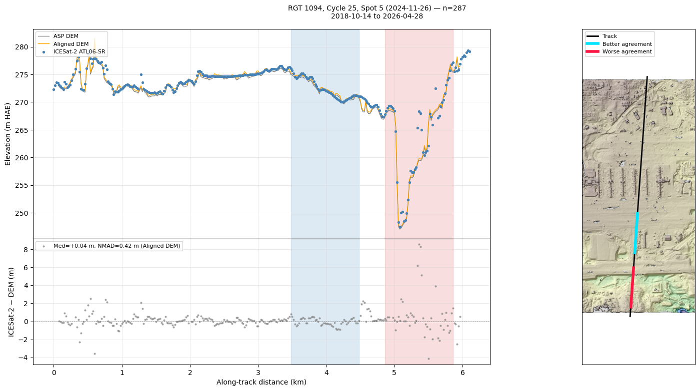
# Profile along the best ICESat-2 track
icesat.plot_atl06sr_dem_profile(key="all")
icesat.plot_best_worst_segments(key="all")

DEM-to-Altimetry Alignment

We use align_and_evaluate() to run pc_align against the filtered ATL06-SR points and automatically decide whether to keep the aligned DEM. The aligned DEM is retained only when:

• Enough ICESat-2 points are available (at least minimum_points)

• The translation magnitude exceeds min_translation_threshold times the DEM GSD

• The median residual p50 improves by more than improvement_threshold_pct percent

On success, the aligned DEM is written to disk and the icesat_minus_aligned_dem column is populated so the comparison plots below can show both pre- and post-alignment distributions. The translation components (north_shift, east_shift, down_shift) and pre/post percentiles (p16_beg/end, p50_beg/end, p84_beg/end) are reported in meters.

# Run pc_align against ICESat-2 and decide whether to keep the aligned DEM.
# minimum_points=100 is used here because ATL06-SR coverage over this ROI
# is sparse; raise it back toward the default 500 for larger scenes.
align_result = icesat.align_and_evaluate(
    processing_level="all",
    minimum_points=100,
    improvement_threshold_pct=5.0,
)
print(f"Status: {align_result.status}")
print(align_result.message)

Writing out: /Users/ben/Desktop/asp-plot-examples/atlanta_stereo_22deg_0d/stereo_no_mapproj/run-DEM_pc_align_translated.tif


Wrote out all aligned DEM to /Users/ben/Desktop/asp-plot-examples/atlanta_stereo_22deg_0d/stereo_no_mapproj/run-DEM_pc_align_translated.tif

Status: success
p50 improved from 0.53 m -> 0.41 m (23.5% reduction). Aligned DEM written to /Users/ben/Desktop/asp-plot-examples/atlanta_stereo_22deg_0d/stereo_no_mapproj/run-DEM_pc_align_translated.tif.

icesat.alignment_report_df

	key	p16_beg	p50_beg	p84_beg	p16_end	p50_end	p84_end	north_shift	east_shift	down_shift	translation_magnitude
0	all	0.178865	0.531587	2.17612	0.105589	0.40661	2.1849	-0.192681	-0.062745	0.290354	0.354074

Aligned DEM Comparison Plots

When alignment succeeds, we can re-render the histogram, profile, and best/worst segment plots with plot_aligned=True to compare the pre-alignment (original DEM) and post-alignment distributions side-by-side. These are the same plots included on the final pages of the PDF report.

# Pre- vs post-alignment histogram with per-landcover statistics
icesat.histogram_by_landcover(key="all", plot_aligned=True)

# Profile along the best ICESat-2 track with the aligned DEM overlaid
icesat.plot_atl06sr_dem_profile(key="all", plot_aligned=True)

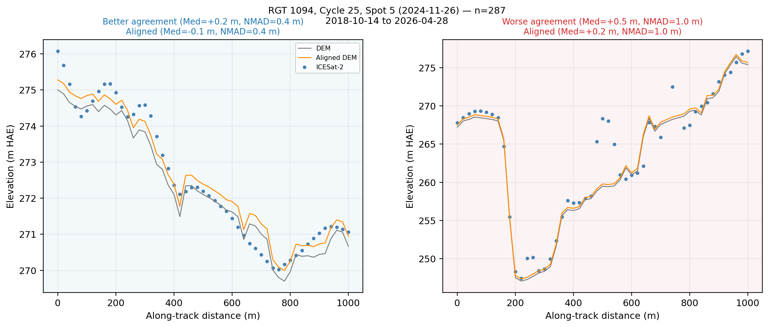
# Best- and worst-agreement segments with the aligned DEM overlaid
icesat.plot_best_worst_segments(key="all", plot_aligned=True)

---

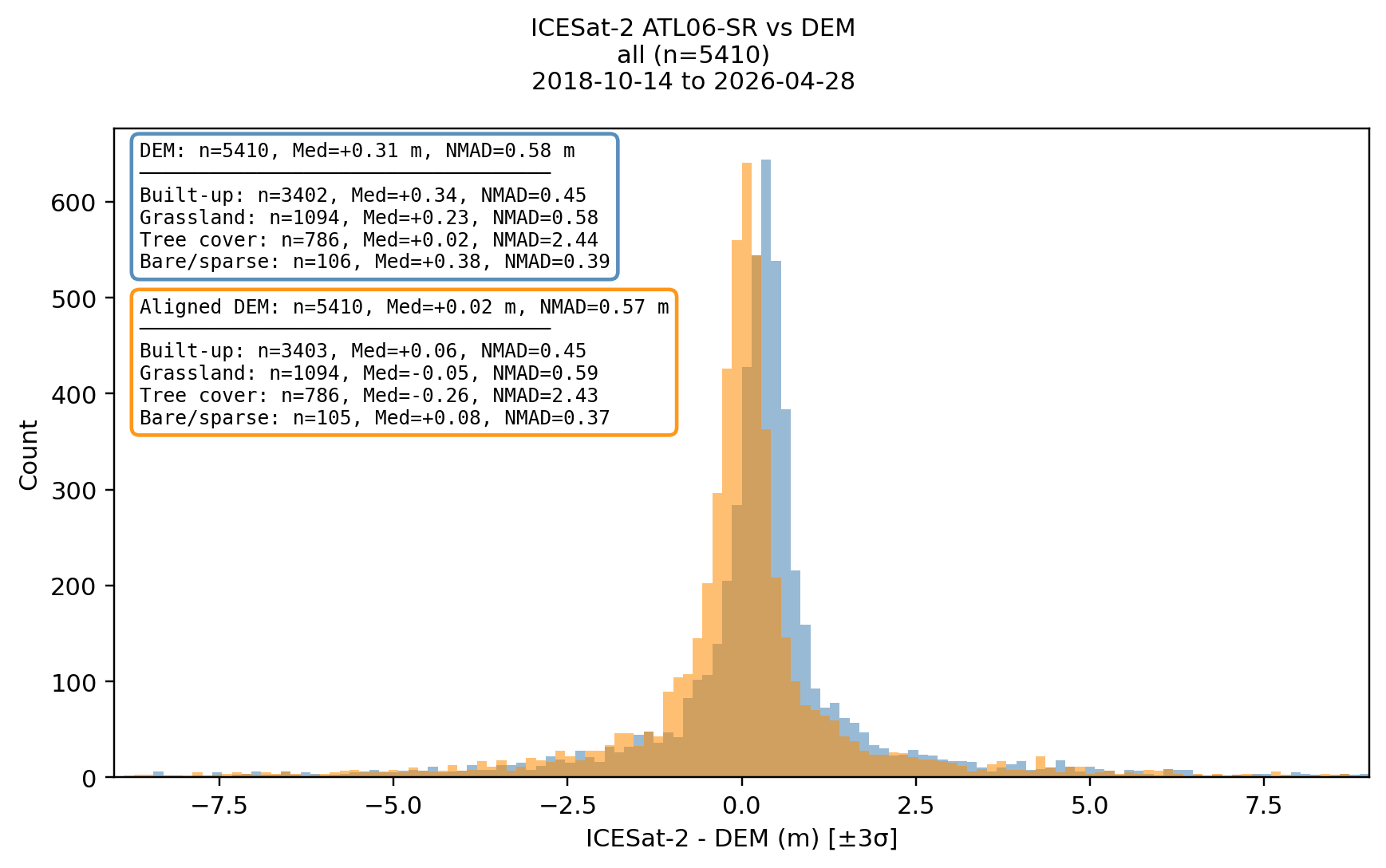
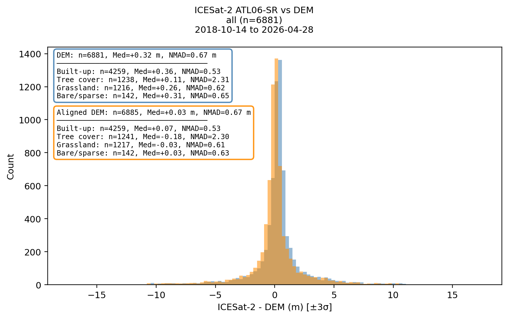
Comparison: ICESat-2 Histograms With vs. Without Mapprojection

The histograms below compare the per-landcover-class ICESat-2 ATL06-SR validation for the same Atlanta stereopair, processed with and without mapprojection. Both DEMs were produced from the same bundle-adjusted input cameras (ba/), so the only difference between the two runs is the mapprojection step. Compare the median bias and NMAD across landcover classes to see the effect.

With Mapprojection

Without Mapprojection

---

Next Steps

This notebook demonstrated the no-mapprojection stereo workflow on the same WorldView-2 stereopair processed in the main Atlanta notebook. For more context and advanced processing:

• Mapprojected workflow: see worldview_spacenet_atlanta_stereo.ipynb for the recommended mapprojected workflow on the same pair.

• Scene selection: see worldview_spacenet_atlanta_stereo_scene_selection.ipynb for the pair-ranking analysis and the DEM-vs-ICESat-2 comparison across all three attempted pairs.

• Jitter correction: For highest-quality DEMs, apply jitter correction following ASP Documentation Section 16.39.9.