WorldView Stereopair Processing: SpaceNet UCSD Example

WorldView Stereopair Processing: SpaceNet UCSD Example#

This notebook demonstrates a stereo processing workflow for WorldView-3 satellite imagery using the NASA Ames Stereo Pipeline (ASP) on a pair selected from the IARPA CORE3D SpaceNet UCSD dataset.

Pair used below:

catid	date	off-nadir (°)
`1040010007A93700`	2015-02-12	8.4	left
`1040010007CA4D00`	2015-02-24	12.9	right

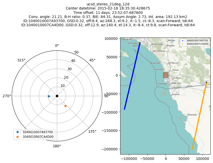
Pair geometry (from StereopairMetadataParser):

Convergence angle: 21.21°
Base-to-height ratio: 0.37
BIE angle: 84.31° (ideal 90°)
Asymmetry angle: 2.73° (ideal 0°)
Temporal separation: 12 days
Sun-elevation delta: 3.1°
Intersection overlap: 94.8%

Why this pair?#

UCSD is a mixed landscape — campus and residential buildings plus coastal valleys and hills — so we target a ~15–25° convergence angle: enough base-to-height to constrain heights over the natural portions, but not so wide that occlusion dominates on building facades. This pair was selected from three attempted WorldView-3 pairs in the companion scene-selection notebook; see section 8 of that notebook for the DEM-vs-ICESat-2 comparison across all three attempts and the rationale for choosing this one.

Processing Overview#

Data Retrieval — Download WorldView-3 imagery from AWS S3
Reference DEM Preparation — Obtain the Copernicus 30m DEM with ellipsoid heights (WGS84)
Bundle Adjustment — Camera model refinement on full images
Mapprojection — Project images onto reference DEM over the 3 × 3 km ROI
Stereo Processing — Generate DEM from the stereopair
Visualization with asp_plot — Plots, ICESat-2 comparison, PDF report

Data Retrieval#

The full catalogue of WV3 scenes and the pair-selection analysis is documented in the companion notebook worldview_spacenet_ucsd_stereo_scene_selection.ipynb. This notebook processes the 21deg_12d pair chosen there.

Download Commands#

Create a working directory and download the NTF images and metadata archives:

$ mkdir -p ucsd_stereo_21deg_12d/images
$ cd ucsd_stereo_21deg_12d/images

# Image 1: 2015-02-12, off-nadir (8.4°), WV3, catid 1040010007A93700
$ aws s3 --no-sign-request cp \
  s3://spacenet-dataset/Hosted-Datasets/CORE3D-Public-Data/Satellite-Images/UCSD/WV3/PAN/12FEB15WV031300015FEB12183926-P1BS-500647760030_01_P001_________AAE_0AAAAABPABS0.NTF .
$ aws s3 --no-sign-request cp \
  s3://spacenet-dataset/Hosted-Datasets/CORE3D-Public-Data/Satellite-Images/UCSD/WV3/PAN/12FEB15WV031300015FEB12183926-P1BS-500647760030_01_P001_________AAE_0AAAAABPABS0.tar .

# Image 2: 2015-02-24, off-nadir (12.9°), WV3, catid 1040010007CA4D00
$ aws s3 --no-sign-request cp \
  s3://spacenet-dataset/Hosted-Datasets/CORE3D-Public-Data/Satellite-Images/UCSD/WV3/PAN/24FEB15WV031300015FEB24183134-P1BS-500647759040_01_P001_________AAE_0AAAAABPABS0.NTF .
$ aws s3 --no-sign-request cp \
  s3://spacenet-dataset/Hosted-Datasets/CORE3D-Public-Data/Satellite-Images/UCSD/WV3/PAN/24FEB15WV031300015FEB24183134-P1BS-500647759040_01_P001_________AAE_0AAAAABPABS0.tar .

# Extract metadata from tars
$ for f in *.tar; do tar xf "$f"; done

After extraction, the NTF and XML files are renamed to <CATID>_P001.{NTF,xml} at the top level of the working directory, which keeps the ASP command invocations below short and explicit.

Stereo Geometry Analysis#

Before processing, it’s useful to analyze the stereo acquisition geometry to verify the convergence angle and other geometric properties. We use asp_plot to visualize the geometry from the XML camera metadata:

# Set the base directory for your processing
directory = "~/Desktop/asp-plot-examples/ucsd_stereo_21deg_12d/"

# Create geometry plotter and auto-detect UTM projection and scene extent from XML metadata
from asp_plot.stereo_geometry import StereoGeometryPlotter

sgp = StereoGeometryPlotter(directory)
utm_code = sgp.get_pair_utm_epsg()
map_crs = f"EPSG:{utm_code}"
scene_bounds = sgp.get_scene_bounds()

print(f"Auto-detected UTM projection: {map_crs}")
print(f"Scene extent (lon/lat): {scene_bounds[0]:.6f} {scene_bounds[1]:.6f} {scene_bounds[2]:.6f} {scene_bounds[3]:.6f}")

# Generate the geometry plot
sgp.dg_geom_plot()

Auto-detected UTM projection: EPSG:32611
Scene extent (lon/lat): -117.294856 32.805385 -117.148296 32.942878

../../_images/cb52f882efddf61af6cf3750809fcfcca97f17e9f855618064f8fed8ccd930de.png

Satellite Position and Orientation Data#

The XML camera metadata also contains ephemeris (position/velocity) and attitude (orientation quaternion) data reported by the satellite during acquisition. Visualizing this data can help assess the quality of the raw metadata before ASP processing.

sgp.satellite_position_orientation_plot()

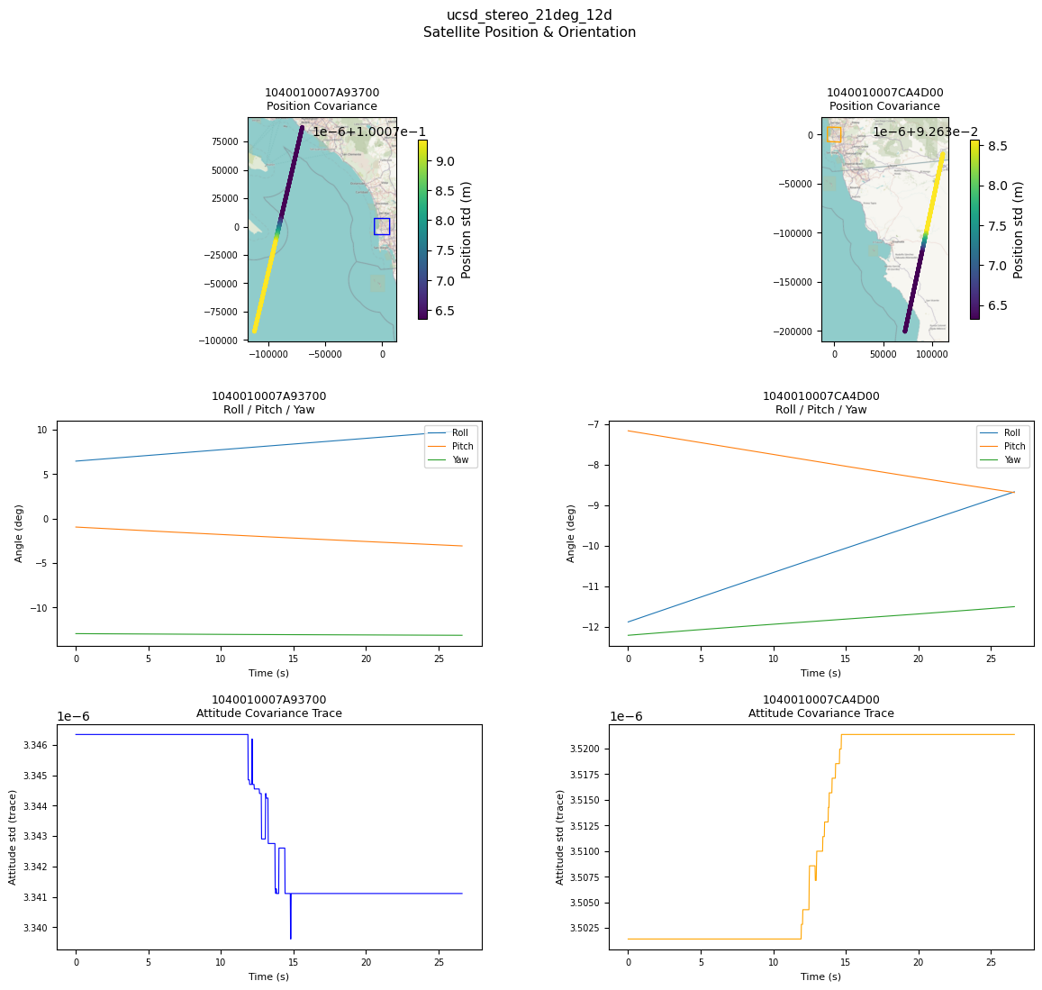
../../_images/8d4132028815041884ee35404c7c861f2c2a0dd66dc4e4b5b0d46c44d719eb75.png

In the above plot:

Top row (Position Covariance): A map showing the satellite’s path over the ground during image capture, colored by how uncertain the satellite’s reported position is (in meters). Lower values mean the satellite knows where it is more precisely.
Middle row (Roll / Pitch / Yaw): Shows how the satellite’s pointing deviates from its expected nadir-pointing orientation over time. Roll is rotation around the flight direction, pitch is rotation around the cross-track axis, and yaw is rotation around the nadir axis. Values near zero mean the satellite is pointing straight down. These are computed by comparing the raw attitude quaternions against a reference orientation estimated from the satellite’s orbital position and velocity.
Bottom row (Attitude Covariance Trace): Shows how uncertain the satellite’s orientation knowledge is over time. Lower values mean the satellite is more confident about which direction it’s pointing. Spikes or jumps indicate moments of less reliable pointing knowledge, which could affect image quality in those portions of the scene.

CCD Artifact Correction — Not Needed for WorldView-3#

The wv_correct tool is used to correct subpixel CCD boundary misalignment artifacts in WorldView-1 and WorldView-2 imagery. These artifacts manifest as discontinuities in DEMs at CCD boundaries.

WorldView-3 does not suffer from the same CCD boundary artifacts, so wv_correct is not needed for this dataset and we skip this step entirely.

For comparison, see the Atlanta example where wv_correct is applied to WorldView-2 imagery.

Processing Configuration#

$ cd ucsd_stereo_21deg_12d

# Target spatial reference system (UTM Zone 11N for San Diego)
$ t_srs="EPSG:32611"

# Processing ROI: 3 × 3 km over UCSD campus + Mount Soledad
$ t_projwin="476000 3635600 479000 3638600"

# Output resolution for mapproject — use the more nadir image's meanProductGSD
$ tr=0.315

# Reference DEM filename (WGS84 ellipsoid heights, projected to UTM)
$ reference_dem_fn="ref/cop30_ucsd_wgs84_utm.tif"

Reference DEM Preparation#

A reference DEM is required for:

Mapprojecting the input images
Validating the output DEM

We use the Copernicus 30m GLO-30 DEM, which provides global coverage with good accuracy.

Download Copernicus DEM with Ellipsoid Heights#

We download with fetch_dem. This requires a free OpenTopography API key.

Important: We use -demtype COP30_E to download the DEM with WGS84 ellipsoid heights directly. ASP requires heights relative to the WGS84 ellipsoid.

The -extent argument uses the scene_bounds from the auto-detected union of both image footprints above. Ensure that the extent has full coverage over the area you are attempting to process.

$ cd ucsd_stereo_21deg_12d

# Download Copernicus DEM with ellipsoid heights (COP30_E)
$ python /path/to/your/fetch_dem/download_global_DEM.py \
  -demtype COP30_E \
  -extent "$scene_bounds" \
  -out_fn "$reference_dem_fn" \
  -out_proj "$t_srs" \
  -apikey [YOUR_OPEN_TOPOGRAPHY_API_KEY]

This creates the reference DEM at ref/cop30_ucsd_wgs84_utm.tif with WGS84 ellipsoid heights in UTM Zone 11N projection.

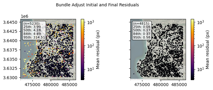
Bundle Adjustment#

Bundle adjustment refines camera models by minimizing reprojection errors of matched feature points. Run on the full images (no ROI cropping) so tie points are spread across the whole scene:

$ cd ucsd_stereo_21deg_12d

$ bundle_adjust \
  --threads 8 \
  --ip-per-image 10000 \
  --tri-weight 0.1 \
  --tri-robust-threshold 0.1 \
  --camera-weight 0 \
  1040010007A93700_P001.NTF 1040010007CA4D00_P001.NTF \
  1040010007A93700_P001.xml 1040010007CA4D00_P001.xml \
  -o ba/run

Bundle Adjustment Results#

Visualize the bundle adjustment results to verify the optimization reduced reprojection errors:

from asp_plot.bundle_adjust import ReadBundleAdjustFiles, PlotBundleAdjustFiles
import contextily as ctx

# Define subdirectories
bundle_adjust_directory = "ba/"
stereo_directory = "stereo/"

# Map configuration (map_crs was auto-detected in the geometry cell above)
ctx_kwargs = {
    "crs": map_crs,
    "source": ctx.providers.Esri.WorldImagery,
    "attribution_size": 0,
    "alpha": 0.5,
}

# Read bundle adjustment residuals
ba_files = ReadBundleAdjustFiles(directory, bundle_adjust_directory)
resid_initial_gdf, resid_final_gdf = ba_files.get_initial_final_residuals_gdfs(residuals_in_meters=True)

# Plot residuals before and after optimization
plotter = PlotBundleAdjustFiles(
    [resid_initial_gdf, resid_final_gdf],
    lognorm=True,
    title="Bundle Adjust Initial and Final Residuals"
)
plotter.plot_n_gdfs(
    column_name="mean_residual",
    cbar_label="Mean residual (px)",
    map_crs=map_crs,
    **ctx_kwargs
)

../../_images/6265fc36e1b7e881b8ec526bf84ddd13cce616f3230297419c18370893ad22e3.png

Define Region of Interest#

The full UCSD images are very large (~43,000 x 43,000 pixels each). To make processing tractable, we define a 3 × 3 km ROI covering the UCSD campus plus the steep terrain of Mount Soledad and Torrey Pines to the southwest toward La Jolla. The same ROI is used across all three pair notebooks (14°, 18°, 21°) so their DEMs can be compared directly.

# ROI in UTM Zone 11N (EPSG:32611): xmin ymin xmax ymax
$ t_projwin="476000 3635600 479000 3638600"

The scene-selection notebook verified that this ROI is fully contained in this pair’s image intersection.

# Get the intersection extent in UTM coordinates (from the geometry cell above)
intersection_bounds = sgp.get_intersection_bounds(epsg=utm_code)
t_projwin = f"{intersection_bounds[0]:.0f} {intersection_bounds[1]:.0f} {intersection_bounds[2]:.0f} {intersection_bounds[3]:.0f}"
print(f"Intersection projwin: {t_projwin}")

Intersection projwin: 472552 3630180 486019 3644498

As noted above, we use the ROI t_projwin="476000 3635600 479000 3638600" — a 3 × 3 km window over UCSD campus + Mount Soledad.

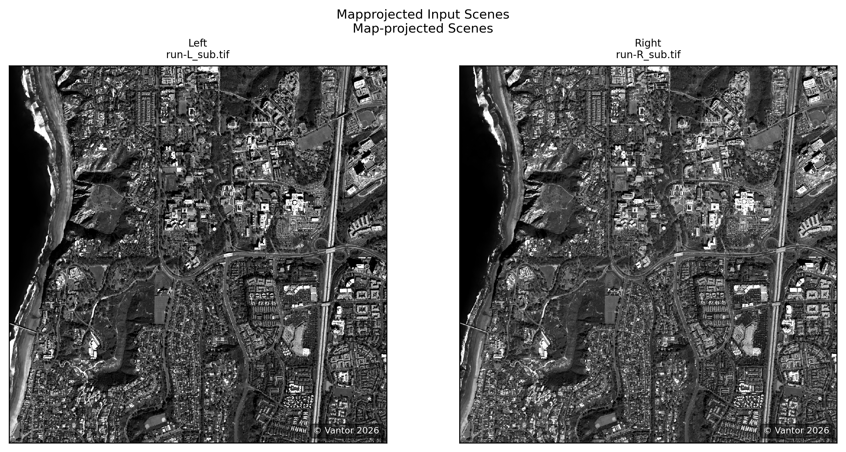
Mapprojection#

Mapproject the two bundle-adjusted images onto the reference DEM over the shared 3 × 3 km ROI:

$ cd ucsd_stereo_21deg_12d

$ mapproject \
  -t rpc --processes 4 --threads 2 \
  --tr $tr --t_projwin $t_projwin --t_srs "$t_srs" \
  --bundle-adjust-prefix ba/run \
  "$reference_dem_fn" \
  1040010007A93700_P001.NTF 1040010007A93700_P001.xml \
  1040010007A93700_P001_map.tif

$ mapproject \
  -t rpc --processes 4 --threads 2 \
  --tr $tr --t_projwin $t_projwin --t_srs "$t_srs" \
  --bundle-adjust-prefix ba/run \
  "$reference_dem_fn" \
  1040010007CA4D00_P001.NTF 1040010007CA4D00_P001.xml \
  1040010007CA4D00_P001_map.tif

Stereo Processing#

$ cd ucsd_stereo_21deg_12d

$ parallel_stereo \
  --stereo-algorithm asp_mgm --subpixel-mode 9 \
  --processes 2 --threads 4 --alignment-method none \
  --bundle-adjust-prefix ba/run \
  1040010007A93700_P001_map.tif 1040010007CA4D00_P001_map.tif \
  1040010007A93700_P001.xml 1040010007CA4D00_P001.xml \
  stereo/run "$reference_dem_fn"

# Generate ~1.2 m DEM (~4× the native input GSD)
$ point2dem --tr 1.2 --t_srs "$t_srs" --errorimage stereo/run-PC.tif

# Difference map vs. reference DEM
$ geodiff stereo/run-DEM.tif "$reference_dem_fn" -o stereo/run_vs_ref

Stereo Results Visualization#

Examine the stereo processing outputs to assess DEM quality:

from asp_plot.stereo import StereoPlotter
from asp_plot.scenes import ScenePlotter

# Plot input scenes (mapprojected images)
scene_plotter = ScenePlotter(directory, stereo_directory, title="Mapprojected Input Scenes")
scene_plotter.plot_scenes()

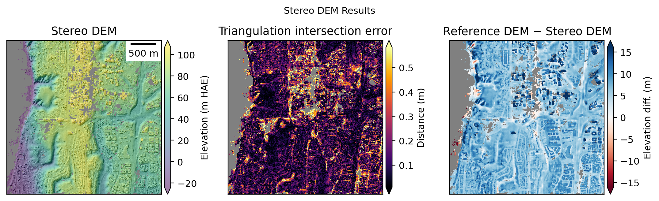
# Plot DEM results
stereo_plotter = StereoPlotter(directory, stereo_directory)
stereo_plotter.title = "Stereo DEM Results"
stereo_plotter.plot_dem_results()

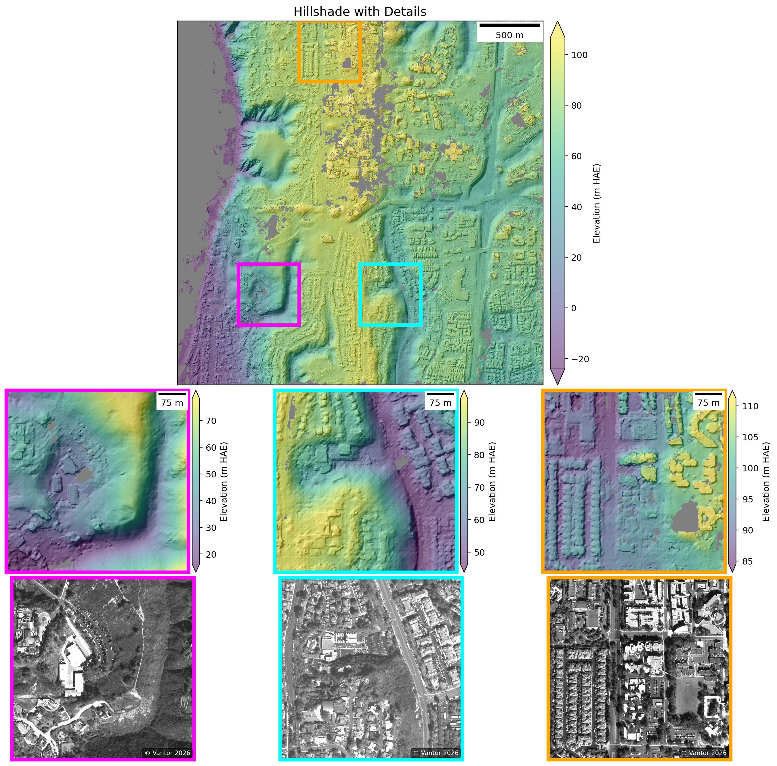
# Plot detailed hillshade with zoom subsets
stereo_plotter.title = "Hillshade with Details"
stereo_plotter.plot_detailed_hillshade(subset_km=0.5)

WARNING:asp_plot.utils:Could not find ('*-align-L.txt',) in /Users/ben/Desktop/asp-plot-examples/ucsd_stereo_21deg_12d/stereo/. Some plots may be missing.

WARNING:asp_plot.utils:Could not find ('*-align-R.txt',) in /Users/ben/Desktop/asp-plot-examples/ucsd_stereo_21deg_12d/stereo/. Some plots may be missing.

Reference DEM: /Users/ben/Desktop/asp-plot-examples/ucsd_stereo_21deg_12d/ref/cop30_ucsd_wgs84_utm.tif

ASP DEM: /Users/ben/Desktop/asp-plot-examples/ucsd_stereo_21deg_12d/stereo/run-DEM.tif

Plotting DEM results. This can take a minute for large inputs.

WARNING:asp_plot.stereo:

Found a DEM of difference: /Users/ben/Desktop/asp-plot-examples/ucsd_stereo_21deg_12d/stereo/run_vs_ref-diff.tif.
Using that for difference map plotting.

../../_images/bf0a64b12aea169287b30b6fe898d2ccc157bd46212d99ffb29b7a807a71f411.png

../../_images/41dd4b63d78530b6a9f394ff6b2474283b3dec94d0adde5a166be116733482f7.png

../../_images/9dc2e32e4661c985761fb885f7c2f54f3eaca2559bff7d4ce7494d6aed0a668d.png

Comprehensive Report and ICESat-2 Altimetry Validation#

In addition to the inline visualizations above, we can validate the ASP DEM against ICESat-2 ATL06-SR altimetry data. This provides an independent accuracy assessment using satellite laser altimetry.

The sections below demonstrate ICESat-2 comparison and generate a comprehensive PDF report.

Setup#

After you have asp_plot installed and ready to use, you can set up the directory and file names:

# Set the base directory for your processing
directory = "~/Desktop/asp-plot-examples/ucsd_stereo_21deg_12d/"

# Define subdirectories for bundle adjustment and stereo results
bundle_adjust_directory = "ba/"
stereo_directory = "stereo/"

Full Report Generation#

Generate a comprehensive PDF report with a single CLI command:

See the resulting report.#

!asp_plot \
  --directory $directory \
  --bundle_adjust_directory $bundle_adjust_directory \
  --stereo_directory $stereo_directory \
  --subset_km 0.25 \
  --report_filename ../../reports/WorldView_UCSD-asp-plot-report.pdf

Processing ASP files in /Users/ben/Desktop/asp-plot-examples/ucsd_stereo_21deg_12d/

Reference DEM: /Users/ben/Desktop/asp-plot-examples/ucsd_stereo_21deg_12d/ref/cop30_ucsd_wgs84_utm.tif

WARNING:asp_plot.utils:Could not find ('*-align-L.txt',) in /Users/ben/Desktop/asp-plot-examples/ucsd_stereo_21deg_12d/stereo/. Some plots may be missing.
WARNING:asp_plot.utils:Could not find ('*-align-R.txt',) in /Users/ben/Desktop/asp-plot-examples/ucsd_stereo_21deg_12d/stereo/. Some plots may be missing.

ASP DEM: /Users/ben/Desktop/asp-plot-examples/ucsd_stereo_21deg_12d/stereo/run-DEM.tif

Using map projection from DEM: EPSG:32611

WARNING:asp_plot.utils:Could not find ('*.[Xx][Mm][Ll]',) in /Users/ben/Desktop/asp-plot-examples/ucsd_stereo_21deg_12d/ba/. Some plots may be missing.

Figure saved to /Users/ben/Desktop/asp-plot-examples/ucsd_stereo_21deg_12d/tmp_asp_report_plots/00.png

Figure saved to /Users/ben/Desktop/asp-plot-examples/ucsd_stereo_21deg_12d/tmp_asp_report_plots/01.png

Figure saved to /Users/ben/Desktop/asp-plot-examples/ucsd_stereo_21deg_12d/tmp_asp_report_plots/02.png

Figure saved to /Users/ben/Desktop/asp-plot-examples/ucsd_stereo_21deg_12d/tmp_asp_report_plots/03.png

Figure saved to /Users/ben/Desktop/asp-plot-examples/ucsd_stereo_21deg_12d/tmp_asp_report_plots/04.png

WARNING:asp_plot.utils:Could not find ('*-mapproj_match_offsets.txt',) in /Users/ben/Desktop/asp-plot-examples/ucsd_stereo_21deg_12d/ba/. Some plots may be missing.

Skipping map-projected residuals plot: 

MapProj Residuals TXT file not found.

WARNING:asp_plot.bundle_adjust:

No reference DEM found in bundle_adjust log. This would only exist if you ran bundle_adjust with the advanced `--mapproj-dem ref_dem.tif` flag. Cannot generate geodiff for /Users/ben/Desktop/asp-plot-examples/ucsd_stereo_21deg_12d/ba/run-initial_residuals_pointmap.csv.

Skipping geodiff plots (requires --mapproj-dem flag in bundle_adjust): 

Geodiff file /Users/ben/Desktop/asp-plot-examples/ucsd_stereo_21deg_12d/ba/run-initial_residuals_pointmap-diff.csv could not be generated. Check that geodiff is installed and a reference DEM was used in bundle_adjust.

Figure saved to /Users/ben/Desktop/asp-plot-examples/ucsd_stereo_21deg_12d/tmp_asp_report_plots/05.png

Plotting DEM results. This can take a minute for large inputs.

WARNING:asp_plot.stereo:

Found a DEM of difference: /Users/ben/Desktop/asp-plot-examples/ucsd_stereo_21deg_12d/stereo/run_vs_ref-diff.tif.
Using that for difference map plotting.

Figure saved to /Users/ben/Desktop/asp-plot-examples/ucsd_stereo_21deg_12d/tmp_asp_report_plots/06.png

Figure saved to /Users/ben/Desktop/asp-plot-examples/ucsd_stereo_21deg_12d/tmp_asp_report_plots/07.png

Detected planetary body: earth

Time filter: 2018-10-14T00:00:00Z to 2026-04-21T00:00:00Z (all available)

ICESat-2 ATL06 request processing for: all
{'poly': [{'lon': -117.25657296374035, 'lat': 32.85824233715243}, {'lon': -117.25657296374035, 'lat': 32.88526799685237}, {'lon': -117.22444511756524, 'lat': 32.88526799685237}, {'lon': -117.22444511756524, 'lat': 32.85824233715243}, {'lon': -117.25657296374035, 'lat': 32.85824233715243}], 't0': '2018-10-14T00:00:00Z', 't1': '2026-04-21T00:00:00Z', 'res': 20, 'len': 40, 'ats': 20, 'fit': {'maxi': 6}, 'cnf': 'atl03_high', 'srt': -1, 'cnt': 10}
Existing file found, reading in: /Users/ben/Desktop/asp-plot-examples/ucsd_stereo_21deg_12d/atl06sr_all.parquet

Filtering ATL06-SR all

  Outlier filter (3σ): all 1148 → 1086 (removed 62)

Figure saved to /Users/ben/Desktop/asp-plot-examples/ucsd_stereo_21deg_12d/tmp_asp_report_plots/08.png

Figure saved to /Users/ben/Desktop/asp-plot-examples/ucsd_stereo_21deg_12d/tmp_asp_report_plots/09.png

Figure saved to /Users/ben/Desktop/asp-plot-examples/ucsd_stereo_21deg_12d/tmp_asp_report_plots/10.png

Figure saved to /Users/ben/Desktop/asp-plot-examples/ucsd_stereo_21deg_12d/tmp_asp_report_plots/11.png

Writing out: /Users/ben/Desktop/asp-plot-examples/ucsd_stereo_21deg_12d/stereo/run-DEM_pc_align_translated.tif

Wrote out all aligned DEM to /Users/ben/Desktop/asp-plot-examples/ucsd_stereo_21deg_12d/stereo/run-DEM_pc_align_translated.tif

Figure saved to /Users/ben/Desktop/asp-plot-examples/ucsd_stereo_21deg_12d/tmp_asp_report_plots/12.png

Figure saved to /Users/ben/Desktop/asp-plot-examples/ucsd_stereo_21deg_12d/tmp_asp_report_plots/13.png

Figure saved to /Users/ben/Desktop/asp-plot-examples/ucsd_stereo_21deg_12d/tmp_asp_report_plots/14.png

Report saved to ../../reports/WorldView_UCSD-asp-plot-report.pdf

ICESat-2 Altimetry Validation#

Compare the ASP DEM with ICESat-2 ATL06-SR altimetry data:

from asp_plot.altimetry import Altimetry

icesat = Altimetry(
  directory=directory,
  dem_fn=stereo_plotter.dem_fn
)

# Request ATL06-SR data (single "all" processing level)
icesat.request_atl06sr_multi_processing(
    processing_levels=["all"],
    save_to_parquet=True,
)

Time filter: 2018-10-14T00:00:00Z to 2026-04-21T00:00:00Z (all available)

ICESat-2 ATL06 request processing for: all
{'poly': [{'lon': -117.25657296374035, 'lat': 32.85824233715243}, {'lon': -117.25657296374035, 'lat': 32.88526799685237}, {'lon': -117.22444511756524, 'lat': 32.88526799685237}, {'lon': -117.22444511756524, 'lat': 32.85824233715243}, {'lon': -117.25657296374035, 'lat': 32.85824233715243}], 't0': '2018-10-14T00:00:00Z', 't1': '2026-04-21T00:00:00Z', 'res': 20, 'len': 40, 'ats': 20, 'fit': {'maxi': 6}, 'cnf': 'atl03_high', 'srt': -1, 'cnt': 10}
Existing file found, reading in: /Users/ben/Desktop/asp-plot-examples/ucsd_stereo_21deg_12d/atl06sr_all.parquet
Filtering ATL06-SR all

# Filter out water bodies
icesat.filter_esa_worldcover(filter_out="water")

No temporal filtering needed for the simplified report workflow. Advanced temporal filtering is still available via:

icesat.predefined_temporal_filter_atl06sr(date=...)
icesat.generic_temporal_filter_atl06sr(select_years=..., select_months=..., ...)

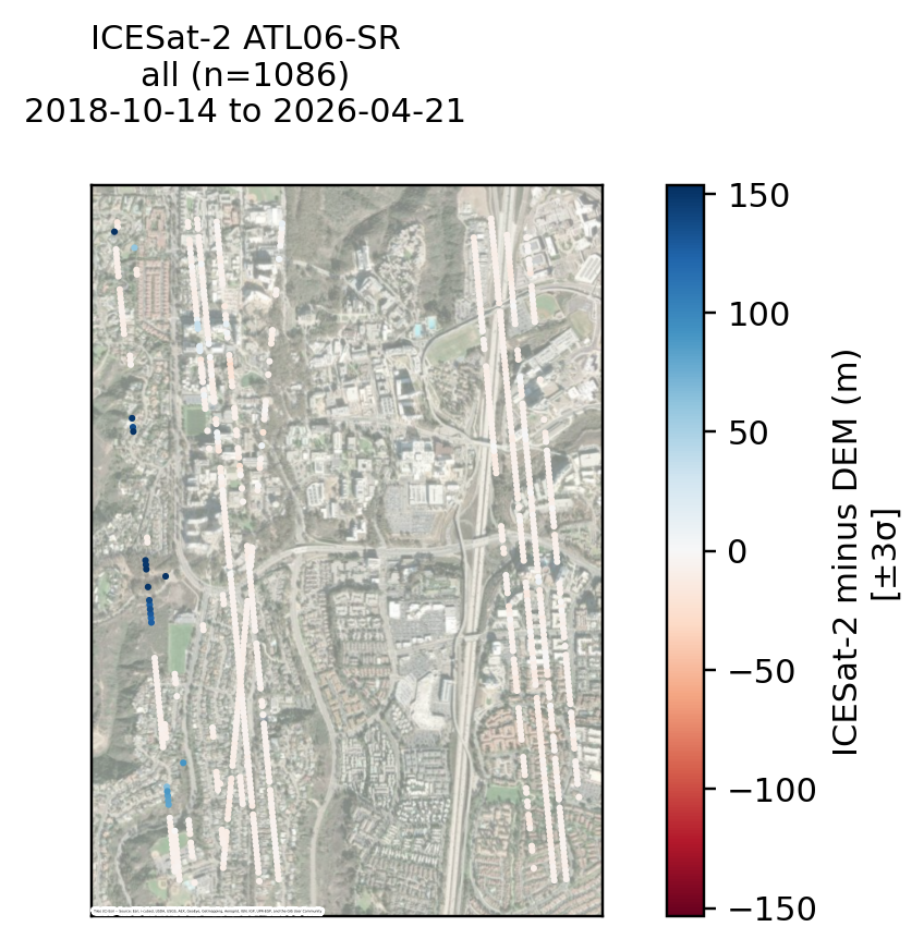
# Map view of ICESat-2 vs DEM differences
icesat.mapview_plot_atl06sr_to_dem(
    key="all",
    map_crs=map_crs,
    **ctx_kwargs,
)

icesat_minus_dem not found in ATL06 dataframe: all. Running differencing first.

  Outlier filter (3σ): all 1148 → 1086 (removed 62)

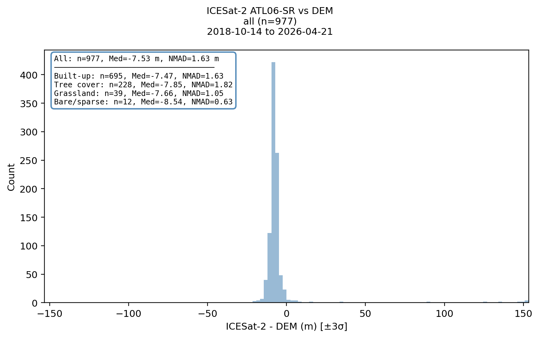
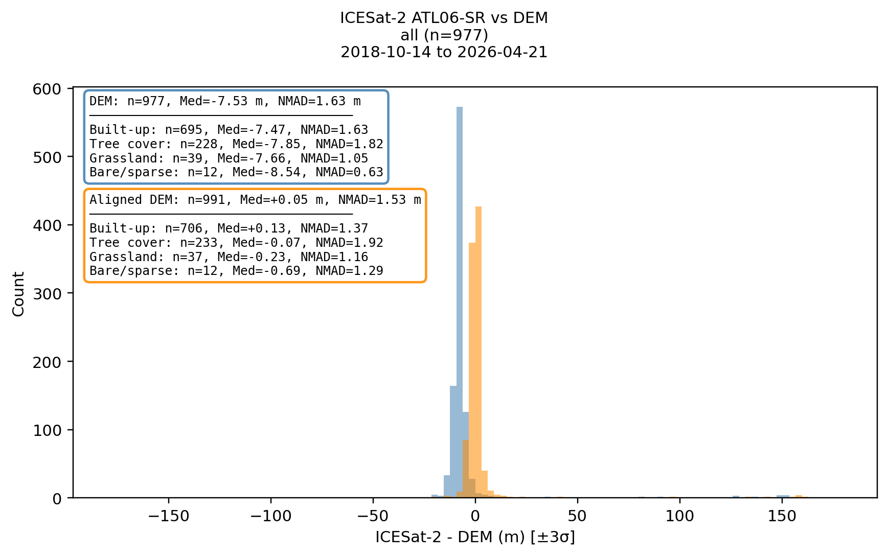
../../_images/0c8d9a5b355a0550508e44e95576ace7b9f314930bcd30805c6eb60129ad247a.png

# Histogram with per-landcover-class statistics
icesat.histogram_by_landcover(key="all")

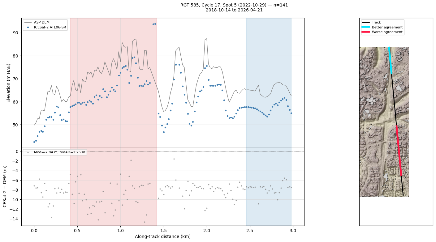
../../_images/0f12bb0429c761ce2e11c1f828adc16d5ff04139515993e9c78e64081efaa568.png

# Profile along the best ICESat-2 track
icesat.plot_atl06sr_dem_profile(key="all")
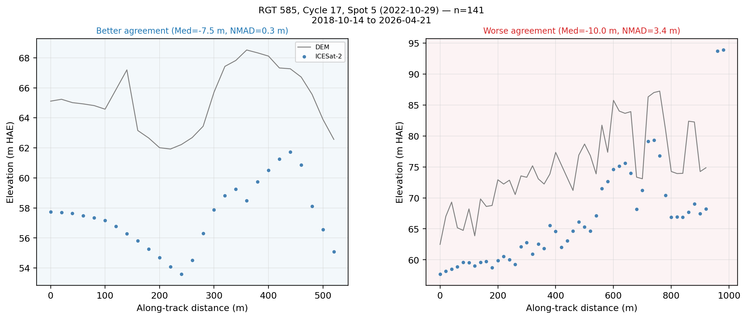
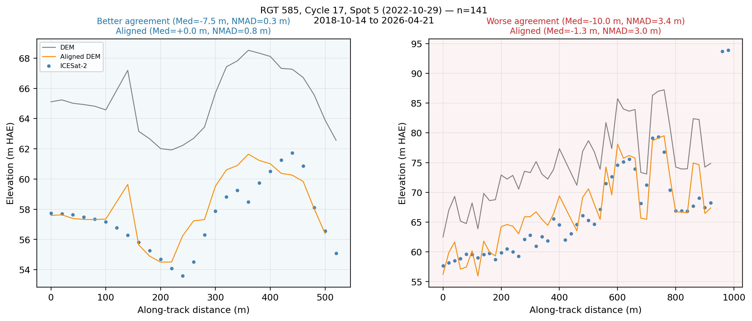
icesat.plot_best_worst_segments(key="all")

../../_images/3887bf45018d56d82944295bc117e14fff4a2aa1597b8bbb0e63cc8a73090f7d.png

../../_images/88001cdd2571d528ade0e664840c286bd3cc4606466328ce3a993be571281301.png

DEM-to-Altimetry Alignment#

We use align_and_evaluate() to run pc_align against the filtered ATL06-SR points and automatically decide whether to keep the aligned DEM. The aligned DEM is retained only when:

Enough ICESat-2 points are available (at least minimum_points)
The translation magnitude exceeds min_translation_threshold times the DEM GSD
The median residual p50 improves by more than improvement_threshold_pct percent

On success, the aligned DEM is written to disk and the icesat_minus_aligned_dem column is populated so the comparison plots below can show both pre- and post-alignment distributions. The translation components (north_shift, east_shift, down_shift) and pre/post percentiles (p16_beg/end, p50_beg/end, p84_beg/end) are reported in meters.

# Run pc_align against ICESat-2 and decide whether to keep the aligned DEM
align_result = icesat.align_and_evaluate(
    processing_level="all",
    improvement_threshold_pct=5.0,
)
print(f"Status: {align_result.status}")
print(align_result.message)

Writing out: /Users/ben/Desktop/asp-plot-examples/ucsd_stereo_21deg_12d/stereo/run-DEM_pc_align_translated.tif

Wrote out all aligned DEM to /Users/ben/Desktop/asp-plot-examples/ucsd_stereo_21deg_12d/stereo/run-DEM_pc_align_translated.tif

Status: success
p50 improved from 7.44 m -> 1.11 m (85.0% reduction). Aligned DEM written to /Users/ben/Desktop/asp-plot-examples/ucsd_stereo_21deg_12d/stereo/run-DEM_pc_align_translated.tif.

icesat.alignment_report_df

	key	p16_beg	p50_beg	p84_beg	p16_end	p50_end	p84_end	north_shift	east_shift	down_shift	translation_magnitude
0	all	5.57724	7.44486	9.3812	0.266115	1.11379	3.67539	0.86893	-2.232433	-7.631565	7.998724

Aligned DEM Comparison Plots#

When alignment succeeds, we can re-render the histogram, profile, and best/worst segment plots with plot_aligned=True to compare the pre-alignment (original DEM) and post-alignment distributions side-by-side. These are the same plots included on the final pages of the PDF report.

# Pre- vs post-alignment histogram with per-landcover statistics
icesat.histogram_by_landcover(key="all", plot_aligned=True)

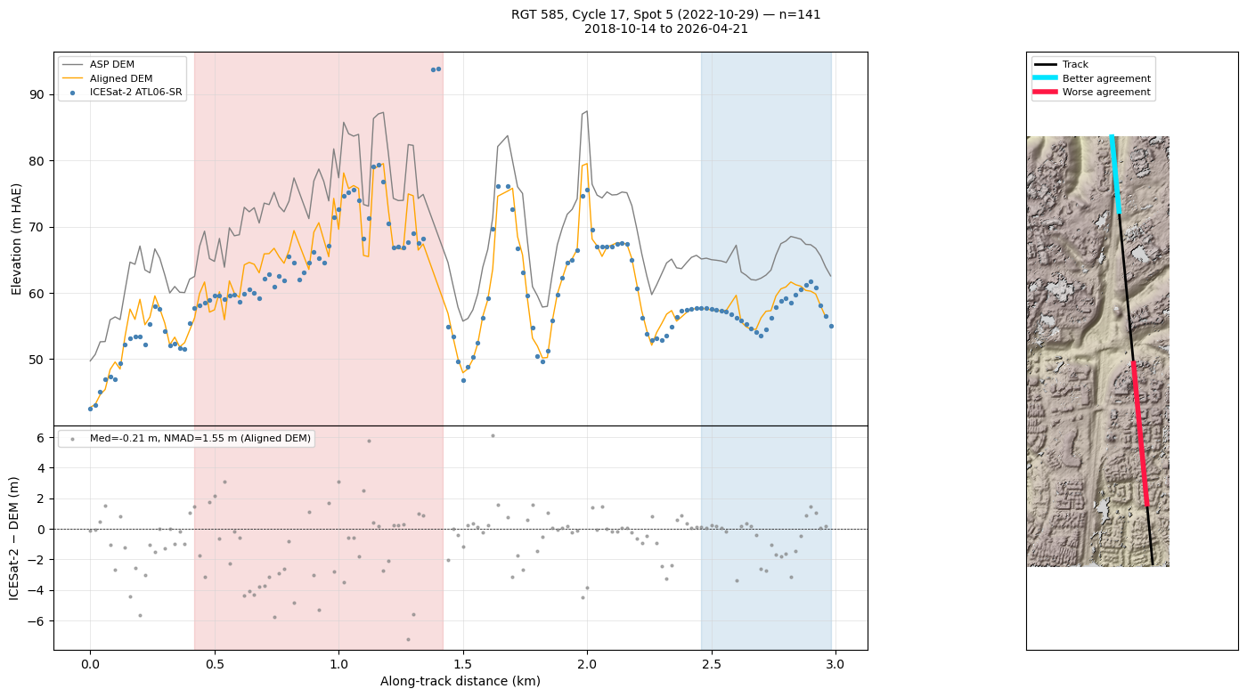
../../_images/c52e3668d1a96074761f1557d026a679a4eccd443ae3984bda0941034abda902.png

# Profile along the best ICESat-2 track with the aligned DEM overlaid
icesat.plot_atl06sr_dem_profile(key="all", plot_aligned=True)

../../_images/0d536e15a5f4373e6a883b6e39053f0be336f85e2c9068d4ea04f3ba714c1ada.png

# Best- and worst-agreement segments with the aligned DEM overlaid
icesat.plot_best_worst_segments(key="all", plot_aligned=True)

../../_images/d2a4a85f4d234d9dd2638657260e91babf58dc3cedf44d1a81ecc4036dcaec52.png

Next Steps#

This notebook demonstrated the end-to-end stereo workflow for a single selected pair. For more context and advanced processing:

Scene selection: see worldview_spacenet_ucsd_stereo_scene_selection.ipynb for the pair-ranking analysis and the DEM-vs-ICESat-2 comparison across all three attempted pairs.
Full-resolution processing: Remove the crop windows to process the entire image overlap (requires significant compute resources).
Jitter correction: For highest-quality DEMs, apply jitter correction following ASP Documentation Section 16.39.9.