WorldView Stereopair Selection: SpaceNet Atlanta Example

This notebook documents the stereo-pair selection analysis used to choose candidate pairs from the SpaceNet Off-Nadir Building Detection Challenge dataset over Atlanta, Georgia.

The goal is to scan the 27 usable WV2 CATIDs hosted under s3://spacenet-dataset/AOIs/AOI_6_Atlanta/metadata/, compute pair geometry with asp_plot.stereopair_metadata_parser, and select pairs with stable imaging geometry for the urban-dominated Atlanta airport processing ROI.

Background: stable imaging geometry

Jeong, J. & Kim, T. (2016), Comparison of positioning accuracy of a rigorous sensor model and two rational function models for weak stereo geometry, ISPRS Journal of Photogrammetry and Remote Sensing 82(8): 625–633 — https://www.sciencedirect.com/science/article/abs/pii/S0099111216301021:

Stable imaging geometry, in addition to a precise sensor model, is also necessary to achieve detailed mapping. The stability of the imaging geometry can be expressed by the values of three angles: the convergence, bisector elevation (BIE), and asymmetry angles. The convergence angle reflects the base-to-height ratio; the BIE angle describes the obliqueness of the epipolar plane; the asymmetry angle specifies the level of symmetry between the left and right observation rays. In the ideal imaging geometry, the epipolar plane would be orthogonal (90° BIE angle) and symmetric (0° asymmetry angle) to the ground plane, to avoid accuracy degradation.

So the ideal is BIE → 90° and asymmetry → 0°. In this notebook these two angles are treated as secondary tiebreakers: they only move a pair up or down the ranking when they are notably far from ideal (BIE ≲ 70°, asymm ≳ 12°).

Convergence target for this scene

Purely urban stereo analyses cite ~5–15° as the ideal convergence range — see Aguilar, M.Á. et al. (2019), 3D modelling of urban structures from very high resolution satellite imagery: a comparative analysis of convergence angle effect, European Journal of Remote Sensing, 52(sup1): 1–13 — https://www.tandfonline.com/doi/full/10.1080/22797254.2018.1551069#abstract. Small convergence reduces occlusion and matching failures on tall, steep-sided building facades.

The Atlanta processing ROI is centered on Hartsfield-Jackson Atlanta International Airport — a mix of flat runway and terminal infrastructure with some residential and wooded areas nearby. As with UCSD, we target ~15–25° convergence to balance occlusion concerns on built-up structures against height precision over flatter terrain:

• Urban-only scenes: ~5–15° is ideal (minimizes building occlusion).

• Natural / low-slope terrain: higher convergence (≳ 25°) is beneficial — the larger base-to-height ratio improves vertical precision where occlusion is not the limiting factor.

• Mixed urban + natural scenes (Atlanta, UCSD): ~15–25° is a practical middle ground.

Single-pass MVS dataset

All 27 Atlanta WV2 CATIDs were acquired on the same orbit pass (2009-12-22, within ~3 minutes of each other). This means temporal separation, solar elevation delta, and solar azimuth delta are effectively zero for every pair. The scoring therefore drops these terms entirely and focuses on:

Priority	Criterion	Direction
Primary	Convergence angle	Target 15–25°
Primary	ROI overlap (containment of the Atlanta airport ROI)	Full containment required
Primary	Off-nadir angle per scene	Smaller (finer GSD, less oblique)
Primary	Sensor consistency	WV2 + WV2 (all Atlanta scenes are WV2)
Secondary	BIE angle	Tiebreaker; penalize only if ≲ 70°
Secondary	Asymmetry angle	Tiebreaker; penalize only if ≳ 12°

---

Atlanta-specific data layout notes

Each CATID’s imagery is tiled into multiple P1BS images (P001, P002, P003, sometimes up to P005). The raw L1B NTFs and tile XMLs live under metadata/<CATID>/<workorder>_<PNNN>_PAN/. For scene selection we only need the XML camera models (satellite/sun angles, footprint polygon), which are very small (~1 MB each). This notebook downloads all tile XMLs for every CATID.

For each CATID the acquisition geometry (sat az/el, sun az/el, GSD) is identical across tiles — they all come from the same satellite pass. The footprint, however, differs per tile. We therefore:

• use the first tile’s XML for the per-scene geometry values,

• union all tile polygons to get the full CATID footprint for overlap analysis.

---

Setup

This notebook only downloads the tile XMLs (very small). It does not download the ~2 GB NTF imagery for any CATID.

import os
import shutil
import subprocess
import tempfile
from itertools import combinations
from pathlib import Path

import contextily as ctx
import geopandas as gpd
import matplotlib.pyplot as plt
import numpy as np
import pandas as pd
from shapely import union_all
from shapely.geometry import box

from asp_plot.stereopair_metadata_parser import StereopairMetadataParser
from asp_plot.utils import get_xml_tag

WORK_DIR = Path("/tmp/atlanta_scene_selection")
XML_DIR = WORK_DIR / "xmls"
FLAT_DIR = WORK_DIR / "flat_xmls"
for d in (WORK_DIR, XML_DIR, FLAT_DIR):
    d.mkdir(parents=True, exist_ok=True)

S3_PREFIX = "s3://spacenet-dataset/AOIs/AOI_6_Atlanta/metadata/"

# Atlanta airport ROI — UTM Zone 16N (EPSG:32616), xmin ymin xmax ymax
# (from worldview_spacenet_atlanta_stereo.ipynb: ~5.7 x 5.4 km over Hartsfield-Jackson)
T_PROJWIN = (735685, 3722295, 741350, 3727695)
UTM_EPSG = 32616

1. Discover CATIDs and download tile XMLs

We look for metadata/<CATID>/ entries (plain catid form, not the duplicated Atlanta_nadirXX_catid_<CATID>/ form — those only hold manifest files). For each CATID we aws s3 cp only the .XML files under its *_PAN/ subdirectories.

# List the plain-CATID subdirectories under metadata/
result = subprocess.run(
    ["aws", "s3", "ls", "--no-sign-request", S3_PREFIX],
    capture_output=True, text=True, check=True,
)
catids = []
for line in result.stdout.strip().splitlines():
    parts = line.split()
    if len(parts) >= 2 and parts[0] == "PRE":
        name = parts[1].rstrip("/")
        # Keep only pure catid dirs (16 hex chars starting with "103")
        if name.startswith("103") and len(name) == 16:
            catids.append(name)

print(f"Found {len(catids)} usable CATIDs.")
for c in catids[:5]:
    print(" ", c)
print("  ...")

Found 27 usable CATIDs.
  10300100023BC100
  1030010002649200
  1030010002B7D800
  103001000307D800
  1030010003127500
  ...

# Download all P1BS XML files under each CATID's PAN tile subdirectories.
# Using s3 sync with --include filters keeps this to only the XMLs (small).
for cid in catids:
    dst = XML_DIR / cid
    if dst.exists() and list(dst.rglob("*.XML")):
        continue  # already downloaded
    dst.mkdir(parents=True, exist_ok=True)
    subprocess.run(
        ["aws", "s3", "--no-sign-request", "sync",
         f"{S3_PREFIX}{cid}/", str(dst),
         "--exclude", "*",
         "--include", "*_PAN/*P1BS*.XML",
         "--only-show-errors"],
        check=True,
    )

# Flatten all CATID-tile XMLs into FLAT_DIR with a name that keeps the CATID:
for cid in catids:
    for xml in (XML_DIR / cid).rglob("*P1BS*.XML"):
        # e.g. 09DEC22163632-P1BS-058332932010_01_P001.XML → <cid>__<original>
        dst = FLAT_DIR / f"{cid}__{xml.name}"
        if not dst.exists():
            shutil.copy(xml, dst)

n_xmls = len(list(FLAT_DIR.glob("*.XML")))
print(f"Tile XMLs on disk: {n_xmls}")

Tile XMLs on disk: 90

2. Extract per-CATID metadata

For each CATID we parse the first tile’s XML for geometry (sat/sun angles, GSD) — these are identical across the tiles of one CATID since they all come from the same pass. The footprint is built by unioning polygons from all tiles of the CATID.

# Dummy parser — we use its instance methods without relying on image_list.
tmp_dir = tempfile.mkdtemp()
any_xmls = sorted(FLAT_DIR.glob("*.XML"))
for x in any_xmls[:2]:
    shutil.copy(x, tmp_dir)
parser = StereopairMetadataParser(tmp_dir)

scene_dicts = []
rows = []

for cid in catids:
    tile_xmls = sorted(FLAT_DIR.glob(f"{cid}__*.XML"))
    if not tile_xmls:
        print(f"skip {cid}: no XMLs")
        continue

    # First tile for geometry values
    rep_xml = str(tile_xmls[0])
    xml_catid = get_xml_tag(rep_xml, "CATID")
    assert xml_catid == cid, f"catid mismatch for {rep_xml}: expected {cid}, got {xml_catid}"

    d = parser.get_id_dict(cid, rep_xml, geteph=True)

    # Replace the single-tile footprint with the union across all tiles
    tile_polys = [parser.xml2poly(str(x)) for x in tile_xmls]
    d["geom"] = union_all(tile_polys)
    d["fp_gdf"] = gpd.GeoDataFrame(
        {"idx": [0], "geometry": d["geom"]}, geometry="geometry", crs="EPSG:4326",
    )

    scene_dicts.append(d)
    rows.append({
        "catid": d["catid"],
        "sensor": d["sensor"],
        "date": d["date"],
        "n_tiles": len(tile_xmls),
        "off_nadir": d["meanoffnadirviewangle"],
        "sat_az": d["meansataz"],
        "sat_el": d["meansatel"],
        "sun_az": d["meansunaz"],
        "sun_el": d["meansunel"],
        "gsd_m": d["meanproductgsd"],
        "cloud": d["cloudcover"],
    })

scene_df = pd.DataFrame(rows).sort_values("date").reset_index(drop=True)
print(f"{len(scene_df)} scenes parsed.")
scene_df

27 scenes parsed.

	catid	sensor	date	n_tiles	off_nadir	sat_az	sat_el	sun_az	sun_el	gsd_m	cloud
0	103001000392F600	WV02	2009-12-22 16:35:10.817775	3	33.5	2.8	52.0	163.6	31.3	0.65	0.02
1	1030010003315300	WV02	2009-12-22 16:35:20.904975	3	30.1	1.1	55.9	163.6	31.3	0.60	0.02
2	103001000307D800	WV02	2009-12-22 16:35:31.393775	3	26.5	358.8	60.3	163.6	31.3	0.57	0.01
3	1030010003127500	WV02	2009-12-22 16:35:41.879575	3	22.4	355.5	64.9	163.7	31.3	0.54	0.01
4	1030010002649200	WV02	2009-12-22 16:35:52.762175	3	18.1	350.3	69.8	163.7	31.3	0.51	0.01
5	1030010002B7D800	WV02	2009-12-22 16:36:00.344175	3	13.7	342.2	74.8	163.8	31.2	0.49	0.00
6	1030010003993E00	WV02	2009-12-22 16:36:10.258375	3	11.2	332.0	77.6	163.8	31.3	0.48	0.01
7	1030010003D22F00	WV02	2009-12-22 16:36:21.288575	3	8.1	304.5	81.0	163.9	31.3	0.48	0.01
8	10300100023BC100	WV02	2009-12-22 16:36:32.488575	3	8.0	263.8	81.0	163.9	31.3	0.48	0.01
9	1030010003CAF100	WV02	2009-12-22 16:36:39.943775	3	10.7	236.5	77.9	164.0	31.3	0.48	0.00
10	10300100039AB000	WV02	2009-12-22 16:36:50.942575	3	14.9	222.6	73.1	164.0	31.3	0.50	0.00
11	1030010003C92000	WV02	2009-12-22 16:37:01.942575	3	19.3	215.2	68.0	164.1	31.3	0.52	0.00
12	103001000352C200	WV02	2009-12-22 16:37:12.743375	3	23.6	210.9	63.1	164.1	31.3	0.55	0.00
13	1030010003472200	WV02	2009-12-22 16:37:23.342575	3	27.6	208.1	58.5	164.2	31.3	0.58	0.00
14	10300100036D5200	WV02	2009-12-22 16:37:33.743375	3	31.2	206.1	54.3	164.2	31.3	0.62	0.00
15	1030010003697400	WV02	2009-12-22 16:37:43.043575	3	33.3	205.5	51.9	164.2	31.4	0.65	0.00
16	1030010003895500	WV02	2009-12-22 16:37:53.155775	3	36.3	204.3	48.2	164.3	31.4	0.71	0.00
17	1030010003832800	WV02	2009-12-22 16:38:03.086575	3	39.0	203.3	44.9	164.3	31.4	0.76	0.01
18	10300100035D1B00	WV02	2009-12-22 16:38:13.012175	3	41.4	202.5	41.9	164.3	31.5	0.83	0.00
19	1030010003CCD700	WV02	2009-12-22 16:38:22.760175	3	43.6	201.9	39.1	164.4	31.5	0.90	0.00
20	1030010003713C00	WV02	2009-12-22 16:38:32.503575	3	45.6	201.3	36.6	164.4	31.5	0.98	0.00
21	10300100033C5200	WV02	2009-12-22 16:38:42.051575	4	47.4	200.8	34.2	164.5	31.5	1.07	0.00
22	1030010003492700	WV02	2009-12-22 16:38:51.607775	4	48.9	200.5	32.1	164.5	31.5	1.16	0.00
23	10300100039E6200	WV02	2009-12-22 16:39:01.365175	4	50.4	200.1	30.0	164.6	31.5	1.27	0.00
24	1030010003BDDC00	WV02	2009-12-22 16:39:11.117175	5	51.7	199.8	28.1	164.6	31.5	1.40	0.00
25	1030010003CD4300	WV02	2009-12-22 16:39:21.079775	5	52.9	199.5	26.3	164.6	31.6	1.53	0.00
26	1030010003193D00	WV02	2009-12-22 16:39:28.143375	5	54.2	198.9	24.4	164.7	31.3	1.71	0.00

3. Enumerate all unique pairs and compute geometry metrics

With {N} scenes we have $\binom{{N}}{{2}}$ candidate pairs. For each pair we compute convergence / BH / BIE / asymmetry via parser.pair_dict, plus intersection, temporal delta, solar deltas, and ROI containment.

roi_utm_poly = box(*T_PROJWIN)
roi_latlon_poly = (
    gpd.GeoDataFrame(geometry=[roi_utm_poly], crs=f"EPSG:{UTM_EPSG}")
    .to_crs("EPSG:4326")
    .geometry.iloc[0]
)

pair_rows = []
for d1, d2 in combinations(scene_dicts, 2):
    if d1["date"] > d2["date"]:
        d1, d2 = d2, d1
    pairname = f"{d1['catid']}_{d2['catid']}"
    p = parser.pair_dict(d1, d2, pairname)

    dt_days = p["dt"].total_seconds() / 86400.0
    delta_sun_el = abs(d1["meansunel"] - d2["meansunel"])
    dsun_az = abs(d1["meansunaz"] - d2["meansunaz"])
    delta_sun_az = min(dsun_az, 360 - dsun_az)

    if p["intersection"] is not None:
        roi_contained = p["intersection"].contains(roi_latlon_poly)
        inter_area = p["intersection_area"]
        inter_perc = min(p["intersection_area_perc"])
    else:
        roi_contained = False
        inter_area = None
        inter_perc = None

    pair_rows.append({
        "pairname": pairname,
        "catid1": d1["catid"], "catid2": d2["catid"],
        "date1": d1["date"], "date2": d2["date"],
        "dt_days": round(dt_days, 2),
        "conv_ang": p["conv_ang"],
        "bh_ratio": p["bh"],
        "bie_ang": p["bie"],
        "asymm_ang": p.get("asymmetry_angle"),
        "inter_km2": inter_area,
        "inter_perc_min": inter_perc,
        "roi_contained": roi_contained,
        "off_nadir1": d1["meanoffnadirviewangle"],
        "off_nadir2": d2["meanoffnadirviewangle"],
        "delta_sun_el": round(delta_sun_el, 2),
        "delta_sun_az": round(delta_sun_az, 2),
    })

pair_df = pd.DataFrame(pair_rows)
print(f"Computed {len(pair_df)} pairs.")
print(f"Pairs fully containing the ROI: {pair_df.roi_contained.sum()}")
print(f"Pairs with convergence in 15–25°: {((pair_df.conv_ang >= 15) & (pair_df.conv_ang <= 25)).sum()}")

Computed 351 pairs.
Pairs fully containing the ROI: 351
Pairs with convergence in 15–25°: 54

4. Filter and score

Filters

1. Intersection polygon must fully contain the Atlanta airport ROI (roi_contained == True).

2. Convergence must not be missing.

Scoring

Since all scenes are from a single orbit pass, temporal separation and solar geometry deltas are zero for every pair and are dropped from the scoring formula:

score = 3.0 · conv_penalty            # 0 inside [15, 25°], else distance from that band
      + 0.10 · mean(off_nadir1, off_nadir2)
      + 5.0  · (bie_ang < 70)
      + 5.0  · (asymm_ang > 12)

def conv_penalty(c):
    if 15 <= c <= 25:
        return 0.0
    return float(min(abs(c - 15), abs(c - 25)))

scored = pair_df[pair_df.roi_contained & pair_df.conv_ang.notna()].copy()
scored["conv_penalty"] = scored["conv_ang"].apply(conv_penalty)
scored["bie_flag"] = (scored["bie_ang"] < 70).astype(int)
scored["asymm_flag"] = (scored["asymm_ang"] > 12).astype(int)

scored["score"] = (
    3.0  * scored["conv_penalty"]
  + 0.10 * scored[["off_nadir1", "off_nadir2"]].mean(axis=1)
  + 5.0  * scored["bie_flag"]
  + 5.0  * scored["asymm_flag"]
)

scored = scored.sort_values("score").reset_index(drop=True)
print(f"Candidates after filtering: {len(scored)}")

display_cols = [
    "pairname", "conv_ang", "bie_ang", "asymm_ang",
    "inter_perc_min", "off_nadir1", "off_nadir2", "score",
]
scored[display_cols].head(15)

Candidates after filtering: 351

	pairname	conv_ang	bie_ang	asymm_ang	inter_perc_min	off_nadir1	off_nadir2	score
0	1030010002B7D800_10300100023BC100	15.97	80.37	4.67	89.81	13.7	8.0	1.085
1	1030010003993E00_1030010003CAF100	18.07	81.69	0.10	88.87	11.2	10.7	1.095
2	1030010003D22F00_10300100039AB000	17.93	79.83	6.11	83.90	8.1	14.9	1.150
3	1030010002B7D800_1030010003CAF100	21.77	81.57	2.34	96.09	13.7	10.7	1.220
4	1030010002649200_10300100023BC100	21.53	78.62	6.85	88.35	18.1	8.0	1.305
5	1030010003993E00_10300100039AB000	23.97	81.22	3.07	84.66	11.2	14.9	1.305
6	1030010002649200_1030010003D22F00	15.29	76.34	9.98	87.94	18.1	8.1	1.310
7	1030010003D22F00_1030010003C92000	23.58	77.98	8.93	83.79	8.1	19.3	1.370
8	10300100023BC100_1030010003C92000	17.35	75.58	12.05	83.76	8.0	19.3	6.365
9	1030010003127500_1030010003D22F00	20.58	74.18	12.71	85.86	22.4	8.1	6.525
10	10300100023BC100_103001000352C200	22.56	73.38	14.69	76.35	8.0	23.6	6.580
11	1030010003CAF100_103001000352C200	16.76	70.89	16.97	83.81	10.7	23.6	6.715
12	1030010003127500_10300100023BC100	26.82	76.69	9.58	86.27	22.4	8.0	6.980
13	103001000307D800_1030010003D22F00	25.42	72.08	15.18	83.06	26.5	8.1	7.990
14	1030010003127500_1030010003993E00	14.54	71.58	15.74	88.17	22.4	11.2	8.060

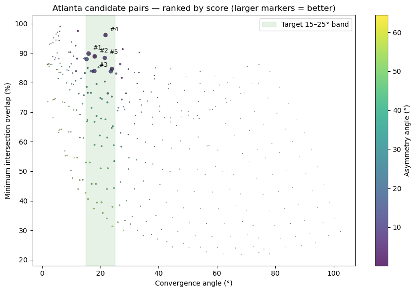
5. Visualize the ranked candidates

fig, ax = plt.subplots(figsize=(9, 6))
sc = ax.scatter(
    scored["conv_ang"], scored["inter_perc_min"],
    c=scored["asymm_ang"], cmap="viridis",
    s=60 * np.clip(1 / (scored["score"] + 0.5), 0, 5),
    alpha=0.8, edgecolor="k", linewidth=0.3,
)
cb = plt.colorbar(sc, ax=ax, label="Asymmetry angle (°)")
ax.axvspan(15, 25, color="green", alpha=0.10, label="Target 15–25° band")
for i in range(min(5, len(scored))):
    row = scored.iloc[i]
    ax.annotate(f"#{i+1}", (row["conv_ang"], row["inter_perc_min"]),
                textcoords="offset points", xytext=(6, 6), fontsize=9)
ax.set_xlabel("Convergence angle (°)")
ax.set_ylabel("Minimum intersection overlap (%)")
ax.set_title("Atlanta candidate pairs — ranked by score (larger markers = better)")
ax.legend(loc="upper right")
plt.tight_layout()
plt.show()

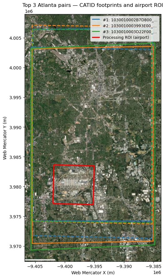
fig, ax = plt.subplots(figsize=(9, 9))

top3_idx = scored.index[:3]
colors = ["tab:blue", "tab:orange", "tab:green"]

for i, (idx, color) in enumerate(zip(top3_idx, colors)):
    row = scored.loc[idx]
    g1 = next(d["geom"] for d in scene_dicts if d["catid"] == row["catid1"])
    g2 = next(d["geom"] for d in scene_dicts if d["catid"] == row["catid2"])
    for g, style in [(g1, "--"), (g2, "-")]:
        gdf = gpd.GeoDataFrame(geometry=[g], crs="EPSG:4326").to_crs(3857)
        gdf.boundary.plot(
            ax=ax, color=color, linestyle=style, linewidth=2,
            label=f"#{i+1}: {row['pairname'][:17]}…" if style == "-" else None,
        )

roi_gdf = gpd.GeoDataFrame(geometry=[roi_utm_poly], crs=f"EPSG:{UTM_EPSG}").to_crs(3857)
roi_gdf.boundary.plot(ax=ax, color="red", linewidth=2.5, label="Processing ROI (airport)")

ctx.add_basemap(ax, crs=3857, source=ctx.providers.Esri.WorldImagery, attribution_size=0)
ax.set_title("Top 3 Atlanta pairs — CATID footprints and airport ROI")
ax.legend(loc="upper right", fontsize=9)
ax.set_xlabel("Web Mercator X (m)")
ax.set_ylabel("Web Mercator Y (m)")
plt.tight_layout()
plt.show()

6. Selected pairs

The top-ranked pairs will be carried forward into companion processing notebooks (to be created). Pair metadata (catids, convergence, etc.) is printed below.

This notebook is also idempotent: re-running after a clean /tmp/atlanta_scene_selection/ wipe will redownload the XMLs from S3.

top3 = scored.head(3)[[
    "pairname", "catid1", "catid2",
    "conv_ang", "bie_ang", "asymm_ang",
    "inter_perc_min", "off_nadir1", "off_nadir2", "score",
]]
top3

	pairname	catid1	catid2	conv_ang	bie_ang	asymm_ang	inter_perc_min	off_nadir1	off_nadir2	score
0	1030010002B7D800_10300100023BC100	1030010002B7D800	10300100023BC100	15.97	80.37	4.67	89.81	13.7	8.0	1.085
1	1030010003993E00_1030010003CAF100	1030010003993E00	1030010003CAF100	18.07	81.69	0.10	88.87	11.2	10.7	1.095
2	1030010003D22F00_10300100039AB000	1030010003D22F00	10300100039AB000	17.93	79.83	6.11	83.90	8.1	14.9	1.150

7. Processing outcomes: DEM-vs-ICESat-2 comparison

We ran the full ASP stereo workflow on the three scene-selected candidate pairs from section 6. All Atlanta SpaceNet scenes are from the same 2009-12-22 acquisition window, so temporal separation is effectively zero for every pair.

For each resulting DEM we compared against ICESat-2 ATL06-SR ground-track points over the ROI. The table below summarizes pre- and post-pc_align height-residual statistics, compiled from a one-off offline run.

Stat columns:

• n_icesat: ATL06-SR points retained after 3σ outlier filtering

• median_dh_pre_m / nmad_dh_pre_m: median and NMAD of ATL06-SR minus DEM before pc_align (meters)

• translation_mag_m (|T|): magnitude of the 3D rigid translation applied by pc_align

• median_dh_post_m / nmad_dh_post_m: same percentiles after alignment

pc_align only solves for a rigid translation, so it is the post-alignment NMAD that gives the cleanest read on intrinsic DEM quality: the median collapses toward zero by construction, and pre-alignment bias reflects absolute positioning rather than DEM geometry.

pair	catid1	catid2	conv (°)	asymm (°)	B/H	n ICESat-2	median pre (m)	NMAD pre (m)	|T| (m)	median post (m)	NMAD post (m)	selected
16deg_0d	1030010002B7D800	10300100023BC100	16.2	5.1	0.28	5429	−0.66	0.72	1.19	0.13	0.71
18deg_0d	1030010003993E00	1030010003CAF100	17.9	0.3	0.31	5401	2.90	0.88	2.95	−0.05	0.88
22deg_0d	1030010002B7D800	1030010003CAF100	21.8	2.6	0.38	5410	0.31	0.58	0.35	0.02	0.57	yes

Why 22deg_0d was selected

• Smallest pre-alignment median bias (+0.31 m) of the three pairs — the DEM was already positioned close to ICESat-2 truth before any correction.

• Smallest translation magnitude (0.35 m) — pc_align only nudged the DEM marginally, confirming the solution is robust in absolute terms.

• Post-alignment NMAD of 0.57 m is the best of the three pairs — the DEM is the most internally consistent after a rigid shift is removed.

• Convergence angle of 21.8° sits in the middle of the 15–25° band targeted in section 4; asymmetry is 2.6°.

The canonical processing notebook worldview_spacenet_atlanta_stereo.ipynb uses this pair (1030010002B7D800 × 1030010003CAF100) and its companion PDF report is at WorldView_Atlanta-asp-plot-report.pdf.

8. Clean up

shutil.rmtree(WORK_DIR, ignore_errors=True)
print(f"Removed {WORK_DIR}: {not WORK_DIR.exists()}")

Removed /tmp/atlanta_scene_selection: True